Defining a region
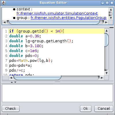
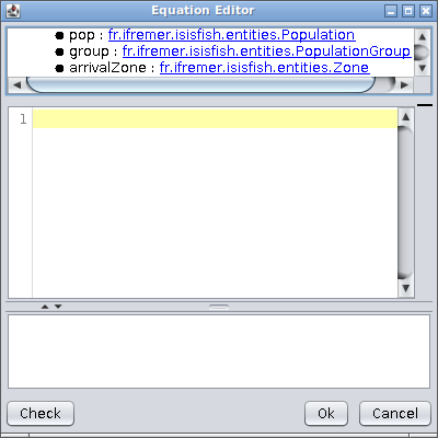
The window for defining regions (the representation of fisheries in ISIS-Fish) can be used to create, view and modify
regions, and all their components. The data defining a region are model parameters in the widest sense of the term and
may be scalars, matrices or equations. Matrices can be edited directly or filled by right clicking a matrix cell,
opening a context menu: using this menu you can Copy/Paste or Import/Export semicolon separated values.
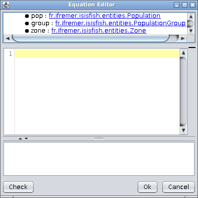
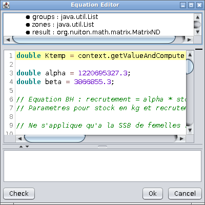
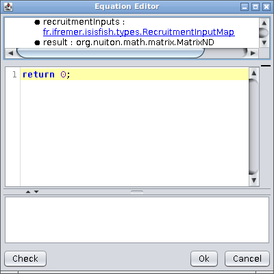
Semicolon separated values can also be copied and pasted directly using Ctrl+C and Ctrl+V. The parameters for an
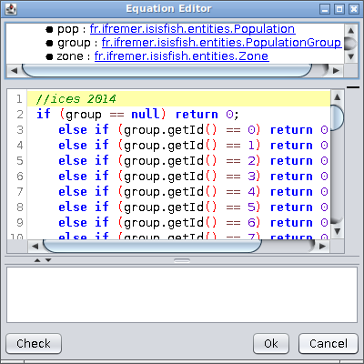
equation can be examined by clicking the adjacent Open editor button. The editor window that opens can also be used
to check the script.
General window layout
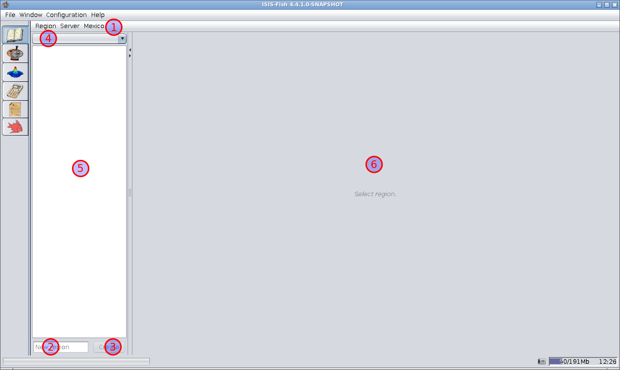
- Region editor menu bar
- The name of a new region to be created
- Button to create a new region
- Dropdown list of regions in the database
- Object tree for the region
- The data entry form
A region represents a fishery.
A new region can be created from scratch by typing the name in the new region field, item 2 above, and then clicking
Create, item 3.
A directory with the new region name will be created and added to the drop down list, item 4 and all the fishery
components will be listed in the object tree, item 5.
A region that has already been created locally or imported can be selected using the drop down list, item 4.
In either case, when a region has been created or selected, a component can be selected in the object tree, item 5, and
defined or modified in the form, item 6.
The form has fields for defining the component’s properties and there may be a map on the right showing the region, the
cells, the zones or the ports.
The region window menu bar
The region window menu bar has menus for manipulating whole regions and objects within regions.
Region menu
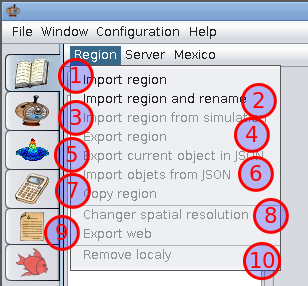
- Import region –
Import a region that has previously been exported from ISIS-Fish.
- Import region and rename –
Import a region that has previously been exported from ISIS-Fish and rename the local copy.
- Import region from simulation –
Import a region from a local simulation. A simulation selection menu will pop up. When the simulation has been
selected, the region name must be specified and then the region is extracted from the simulation and saved locally.
- Export region –
Export the currently selected region as a compressed archive file. The archive may be imported by any copy of
ISIS-Fish v4. A region must already be selected.
- Export current object in JSON –
Exports the currently selected object as a JSON file.
- Import objects from JSON –
Imports one or more objects contained in a JSON file.
- Copy region –
Copies a complete region. A region must already be selected.
- Change spatial resolution –
Changes the spatial resolution for the selected region.
- Export web –
As for “Export region” but sends the archive to a URL.
- Remove locally -
Deletes the local copy of the currently selected region. A region must already be selected. N.B. The delete operation
is irreversible. Once a local copy of a region has been deleted, it cannot be recovered.
Server menu
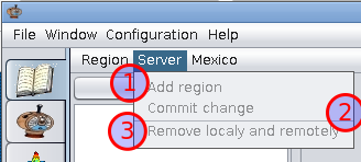
The menu has the actions for backing up a region on the server or removing it from the server.
- Add region –
Backup a new region to the server. A dialog box will request a comment on the backup. When you click OK, the region
is added to the server, provided that you have “write” permission for the server (see VCS Configuration).
- Commit change –
Send you local changes to the server.
- Remove locally and remotely –
Removes the region backup from the server as well as the local copy of the region. N.B. Use with extreme care!
Mexico menu

Create or edit a region
A region is defined in stages :
- Create or select a region
- Define the cells
- Define the zones
- Define the ports
- Define the species
- Define the populations
- Define the fishing gear
- Define the “metiers”
- Define the types of trip
- Define the types of vessel
- Define the sets of vessels
- Define the strategies
3Add observations
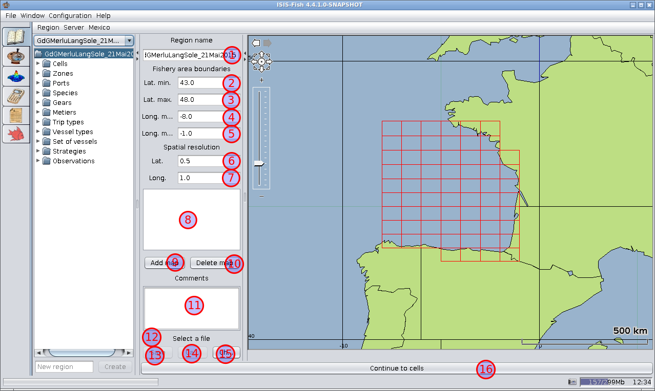
1. Create or select a region
When a region has been created or selected, the general properties of the region are displayed in the form.
Les latitudes et longitudes sont en degrés décimaux.
-
Region name –
The name of the region (as it is the name of the fishery object, it is a good idea to standardize the name, e.g.
using alphanumeric characters and avoiding punctuation). The region is a rectangle (on a Mercator projection) with a
regular array of cells.
-
Lat. min. –
The minimum latitude in degrees North (floating point).
-
Lat. max. –
The maximum latitude in degrees North (floating point).
-
Long. min. –
The minimum longitude in degrees East (floating point).
-
Long. max. –
The maximum longitude in degrees East (floating point).
-
Lat. (Spatial resolution) –
The latitudinal height of each cell (floating point).
-
. Long. (Spatial resolution) –
The longitudinal width of each cell (floating point).
-
List of maps to be used in place of the default world map.
-
Add map –
To add a map to replace the default world map, click Add map and select the file using the dialog box which will be
displayed. The map should be in one of the formats shp, e00, mif, rpf, cadrg, cib, vmap, dcw or vpf.
-
Delete map –
Removes a map that has been previously added.
-
Comments –
Any additional information about the region can be saved as a comment.
-
Select a file –
The region can be set up using a file with a predefined grid. Click …
-
Save –
Once the region has been set up, with maps and predefined grid, if required, the general properties of the region can be saved.
-
Cancel –
Throws away the modifications made to the region and reverts to the previous version.
-
Check –
Checks that the general properties of the region are coherent.
-
Continue to cells –
When the general properties of the region have been defined you can move on to the next step.
Either click Continue to cells or select Cells in the object tree.
2. Define the cells
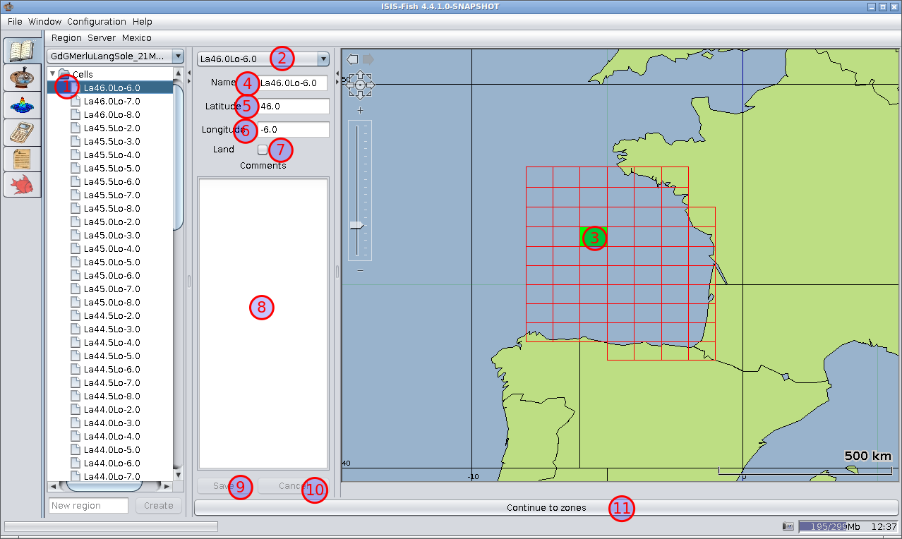
The form for cells allows the user to rename cells, to define them as land and to add comments to each cell.
- Cell in the object tree –
A cell can be selected in the object tree: the selection in the dropdown list and the map will be updated.
- Cell in the dropdown list –
A cell can be selected in the dropdown list: the selection in the object tree and the map will be updated.
- Cell on the map –
A cell can be selected on the map: the selection in the object tree and the dropdown list will be updated.
- Name –
By default the name of the cell is the latitude and longitude of the bottom left-hand corner, for example,
La44.5Lo-3.0. This may be changed by the user.
- Latitude –
Latitude of the left-hand edge of the cell, in degrees. This may not be changed.
- Longitude –
Longitude of the bottom edge of the left hand cell, in degrees. This may not be changed
- Land –
Checkbox to be checked if the cell is on land.
- Comments –
This field is used for adding comments linked to the cell selected. Each cell may have its own comments.
- Save –
Saves the changes to the cell selected. Do not forget to save your changes.
- Cancel –
Throws away the modifications made to the cell and reverts to the previous version.
- Continue to zones –
To move on to the next step either click Continue to zones or select Zones in the object tree
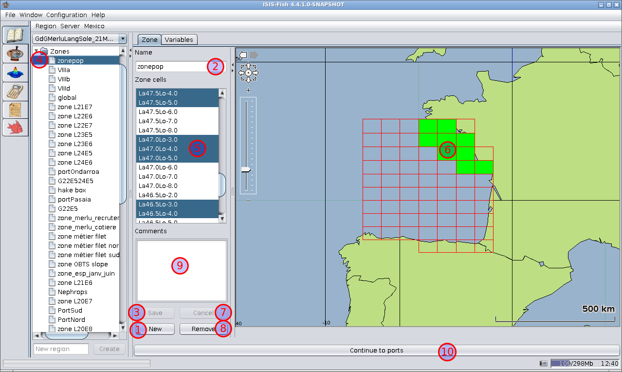
3. Define the zones
Zones, groups of cells, are used to define the limits of populations, “metiers” and fishery management measures, and,
therefore, must be defined first.
-
New –
Creates an empty zone with the name “Zone_new”, adds it to the object tree and displays it for editing.
At this point, the zone has been created: you should now set the name and associate it with one or more cells.
-
Name –
The name of the zone (as it is the name of the fishery object, it is a good idea to standardize the name, e.g. using
alphanumeric characters and avoiding punctuation).
-
Save –
Saves the changes to the zone selected. Do not forget to save your changes.
-
Zone in the object tree :
a zone to be modified must be selected in the object tree.
-
Zone Cells –
Select a single cell by clicking the name. Select a group of cells by clicking the first cell, pressing Shift and
clicking the last cell, Select or unselect individual cells by pressing Ctrl and clicking the cell.
-
Zone Cells on the map :
Select or unselect individual cells by clicking the cell. The cells selected will be highlighted.
-
Cancel –
Throws away the modifications made to the zone and reverts to the previous version.
-
Remove –
Deletes the zone. N.B. The delete operation is irreversible. Once a zone has been deleted, it cannot be recovered.
-
Comments –
This field is used for adding comments linked to the zone selected. Each zone may have its own comments.
-
Continue to ports –
To move on to the next step either click Continue to ports or select Ports in the object tree.
Note. The zones used to define a single population may overlap.
Variables tab
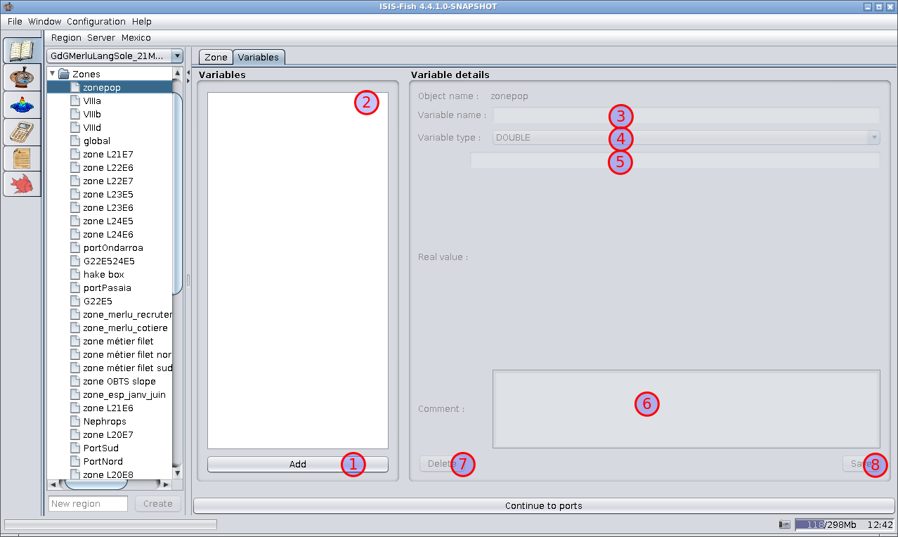
- Add – Adds a variable for this zone with the default name VarName.
- Variables – List of variables defined for this zone.
- Variable name – Name of the variable selected. The name should conform to Java naming standards.
- Variable type – Dropdown list defining the type of variable.
- Variable value – Real (double length floating point), equation or matrix.
- Comment – A description of the variable.
- Delete – Deletes the variable. N.B. The delete operation is irreversible.
- Save – Saves the changes to the variable selected. Do not forget to save your changes.
4. Define the ports
The ports are used to calculate transport costs. A port is defined as being within the cell that encloses the
geographical location of the port.
A port corresponds to just one cell.
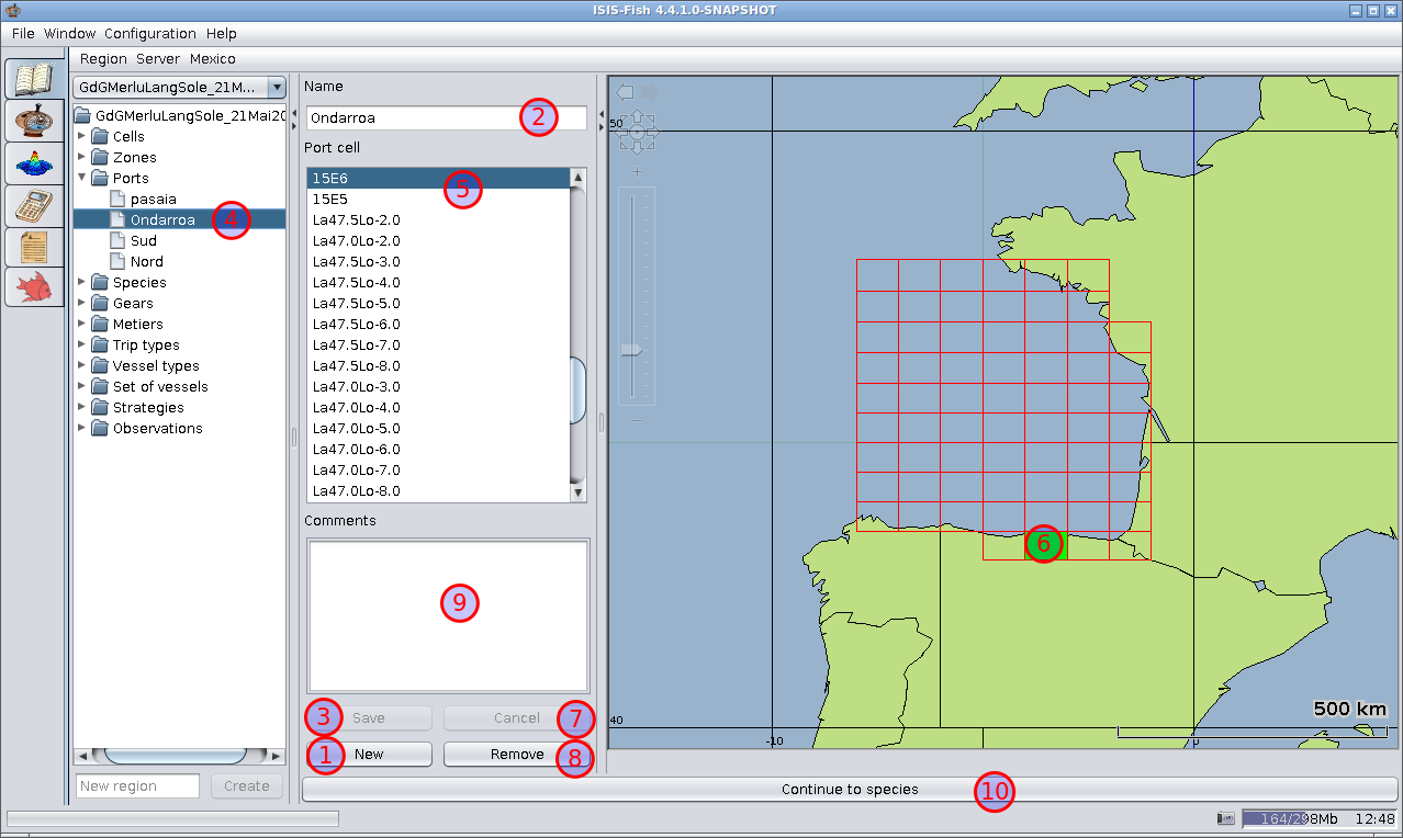
- New – Creates an empty port with the name “Port_new”, adds it to the object tree and displays it for editing.
At this point, the port has been created: you should now set the name and associate it with a cell.
- Name – The name of the port (as it is the name of the fishery object, it is a good idea to standardize the name,
e.g. using alphanumeric characters and avoiding punctuation).
- Save – Saves the changes to the port selected. Do not forget to save your changes.
- Port in the object tree : a port to be modified must be selected in the object tree.
- Port cell – Select a single cell by clicking the name.
- Port cell on the map : Select a cell by clicking it. The cell selected will be highlighted.
- Cancel – Throws away the modifications made to the port and reverts to the previous version.
- Remove – Deletes the port. N.B. The delete operation is irreversible. Once a port has been deleted, it cannot be recovered.
- Comments – This field is used for adding comments linked to the port selected. Each port may have its own comments.
- Continue to species – To move on to the next step either click Continue to species or select Species in the object tree.
5. Define the species

-
New – Creates an empty species with the name “Species_new”, adds it to the object tree and displays it for
editing. At this point, the species has been created: you should now set the name and the other properties.
-
Species name – The common name of the species (as it is the name of the fishery object, it is a good idea to
standardize the name, e.g. using alphanumeric characters and avoiding punctuation).
-
Save – Saves the changes to the species selected. Do not forget to save your changes.
-
Scientific name – The scientific name can be set here, but only the common name is used.
-
Rubin code – The Rubin code (GENUs SPEcies) for the species.
-
CEE – CEE
Most of the biological properties of the species are dependent on the parameter used to define the population
structure which may be either age or length.
-
Age (Structure) – If Age is selected the population dynamics are defined in terms of age groups.
-
Length (Structure) – If Length is selected the population dynamics are defined in terms of length groups
-
Comments – This field is used for adding comments linked to the species selected. Each species may have its own
comments.
-
Cancel – Throws away the modifications made to the species and reverts to the previous version.
-
Remove – Deletes the species. N.B. The delete operation is irreversible. Once a species has been deleted, it
cannot be recovered.
-
Species in the object tree – a species to be modified must be selected in the object tree.
-
Continue to populations – To move on to the next step either click Continue to populations or select
Populations for the species in the object tree.
6. Define the populations
The form for defining a population has eleven tabs. When a new population has been created, define the properties in the
order in which the tabs are described below.
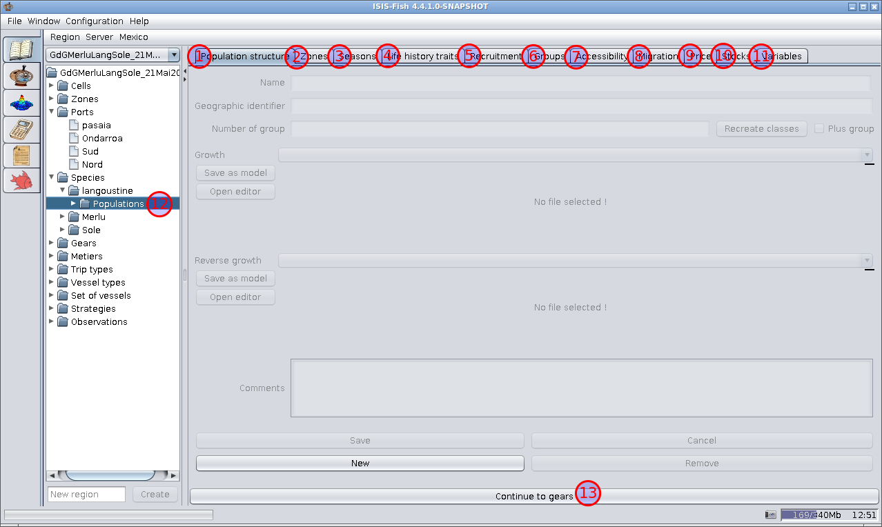
- Population structure tab
- Zones tab
- Seasons tab
- Life history traits tab
- Recruitment tab
- Groups tab
- Accessibility tab
- Migration tab
- Price tab
- Stocks tab
- Variables tab
- Populations in the object tree – a population to be modified must be selected in the object tree.
- Continue to gears – To move on to the next step either click Continue to gears or select Gears in the object tree.
The definition of the population dynamics requires a certain number of equations.
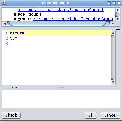
- Growth equation – This is used when the population is age structured. The equation should return
the length (floating point) calculated as a function of age which is given as 12 times the age in years.
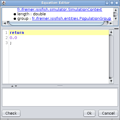
- Reverse growth equation – This is used when the population is length structured. The equation
should return the age (months, floating point) calculated as a function of length.
- Natural death rate equation.
- Fishing gear selectivity equation.
- Reproduction rate equation.
- Fishing mortality, other fleets equation.
Population structure tab
The population structure tab is used to define the biological parameters that apply to the whole population
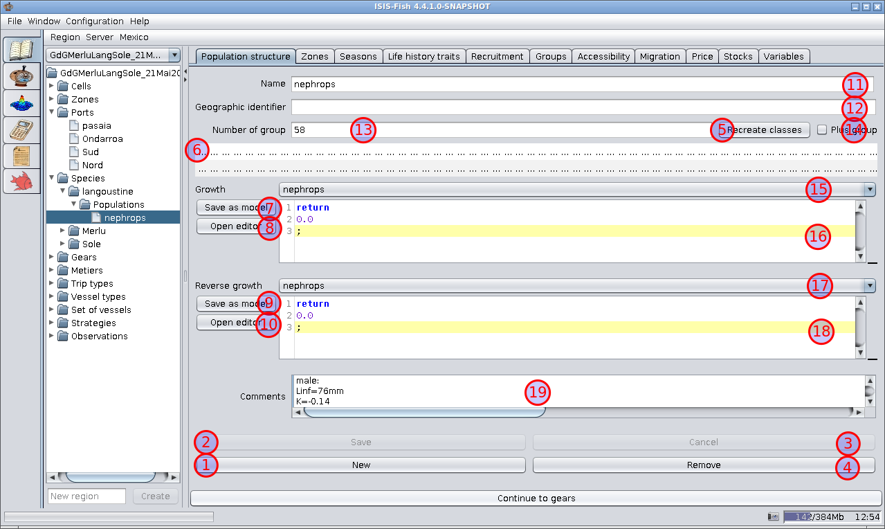
- New – Creates an empty population with the name “Population_new”, adds it to the object tree and displays it for
editing.
- Save – Saves the changes to the population selected. Do not forget to save your changes.
- Cancel – Throws away the modifications made to the population and reverts to the previous version.
- Remove – Deletes the population. N.B. The delete operation is irreversible. Once a population has been deleted,
it cannot be recovered.
- Recreate classes – Creates, or recreates the age or length groups for the population. This opens the “Create
groups” dialog box. The growth or reverse growth equation, depending on whether the population is structured by age
or length, must have been defined. Do not forget to recreate the age or length groups if the growth parameters have
been changed.
- Age or length groups – Displays the age or length groups, in terms of age and length, once the growth, or
reverse growth, have been defined and the groups created.
- Save as model (Growth equation) – Saves the growth equation as a model in the ISIS-Fish scripts – this can be
useful if the equation can be reused for other species.
- Open editor (Growth equation) – Opens the equation editor for editing the growth equation.
- Save as model (Reverse growth equation) – Saves the reverse growth equation as a model in the ISIS-Fish scripts –
this can be useful if the equation can be reused for other species.
- Open editor (Reverse growth equation) – Opens the equation editor for editing the reverse growth equation.
- Name – The name of the population (as it is the name of the fishery object, it is a good idea to standardize the
name, e.g. using alphanumeric characters and avoiding punctuation).
- Geographic identifier – A description that will help to distinguish this population from other populations of the
same species.
- Number of groups – Displays the number of age or length groups created.
- Plus group – Specifies that the distribution is open-ended
- Growth equation selector – Selects a growth equation for the population.
- Growth equation – Displays the growth equation, length as a function of age, for the population. This equation
will only be used if the population is structured by age. If the equation has been selected using the selector, item
15, the parameters may need to be changed to match the specific case. An equation can also be written from scratch
using the equation editor. The equation may be edited in this frame. Although the age is usually expressed in years
(Mature and Age classes) but the parameter “age” for the growth equation is in months.
- Reverse growth equation selector – Selects a reverse growth equation for the population.
- Reverse growth equation – Displays the reverse growth equation, age as a function of length for the population.
This equation will only be used if the population is structured by length. If the equation has been selected using
the selector, item 17, the parameters may need to be changed to match the specific case. An equation can also be
written from scratch using the equation editor. The equation may be edited in this frame. Although the age is usually
expressed in years (Mature and Age classes), the age should be returned in months.
- Comments – This field is used for adding comments linked to the population selected. Each population may have its
own comments.
Zones tab
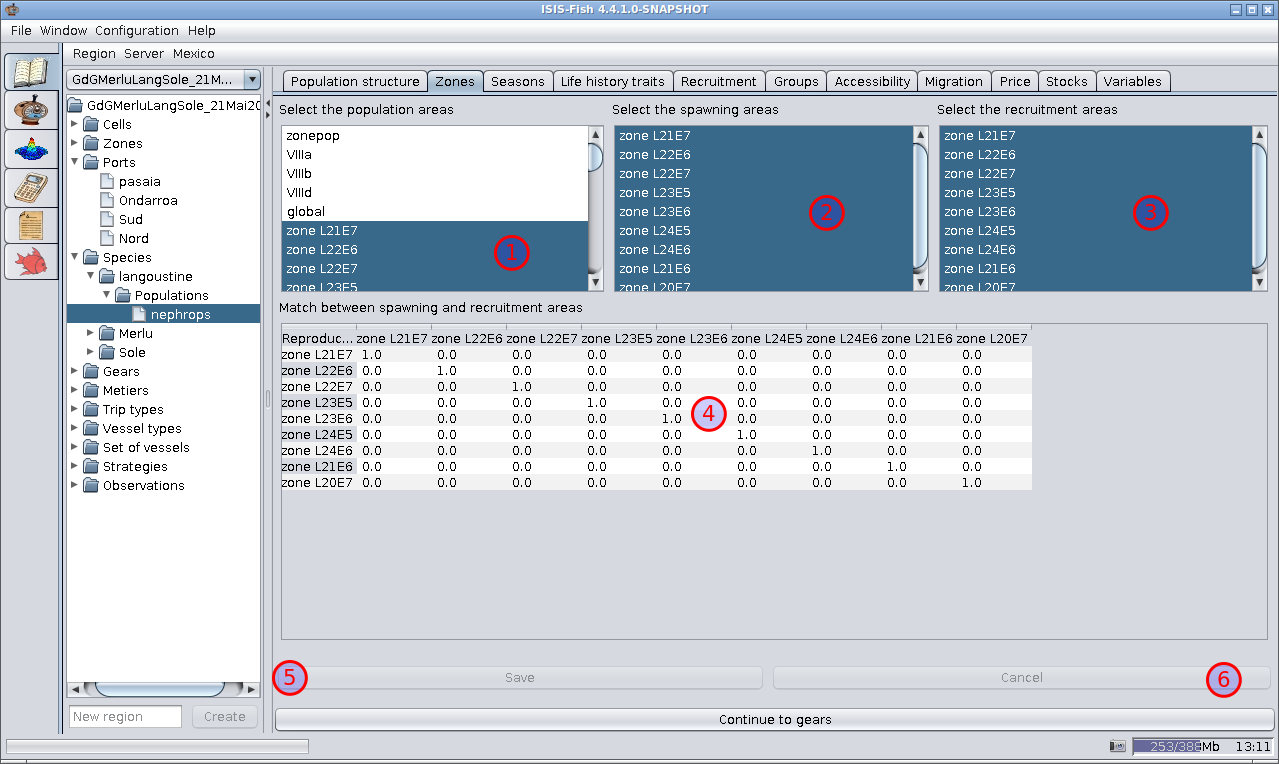
- Select the population areas – This list is used to define the population areas by selecting the zones where the
population is present at some time during the year. Press Ctrl when clicking a zone to select or deselect it.
- Select the spawning areas – This list is used to define the spawning areas by selecting the zones where spawning
takes place. Press Ctrl when clicking a zone to select or deselect it.
- Select the recruitment areas – This list is used to define the recruitment areas by selecting the zones where
recruitment takes place. Press Ctrl when clicking a zone to select or deselect it.
- Match between spawning and recruitment areas – This correspondence matrix defines the fraction of eggs released in
each zone in the spawning area that are recruited in each zone of the recruitment area.
- Save – Saves the changes to the areas for the population. Do not forget to save your changes.
- Cancel – Throws away the modifications made to the areas and reverts to the previous version.
Seasons tab (population structured by age)
The layout of the Seasons tab depends on whether the population is structured by age or length.

- Select a season – A list of all seasons currently defined for the population. Select one to set the properties.
- Season – The season is shown in yellow. The start and end of the season can be adjusted by dragging the ends of
the bar using the mouse, the whole season can be moved by dragging the middle.
- Change of group – Checked if the fish change age or length group at the start of the season. For age structured
populations, there should only be one change per year.
- Reproduction – Checked if the fish spawn in this season. If it is checked, the “Distribution of spawning” matrix
will be displayed.
- Distribution of spawning – Shows the fraction of the annual spawning that takes place in each month. Double click
on a cell to set the fraction. Changes to a cell do not take effect until you press Enter or click another cell in
the matrix. Changes to the matrix should be saved using the Save button.
- Comments – This field is used for adding comments linked to the season selected. Each season may have its own
comments.
- Save – Saves the changes to the season selected. Do not forget to save your changes.
- New – Creates an empty season with a default range of months and displays it for editing.
- Cancel – Throws away the modifications made to the season and reverts to the previous version.
- Remove – Deletes the season. N.B. The delete operation is irreversible. Once a season has been deleted, it cannot
be recovered.
N.B. Ensure that “Change of group” is only checked for one season, otherwise the fish may change group more than once in
a year.
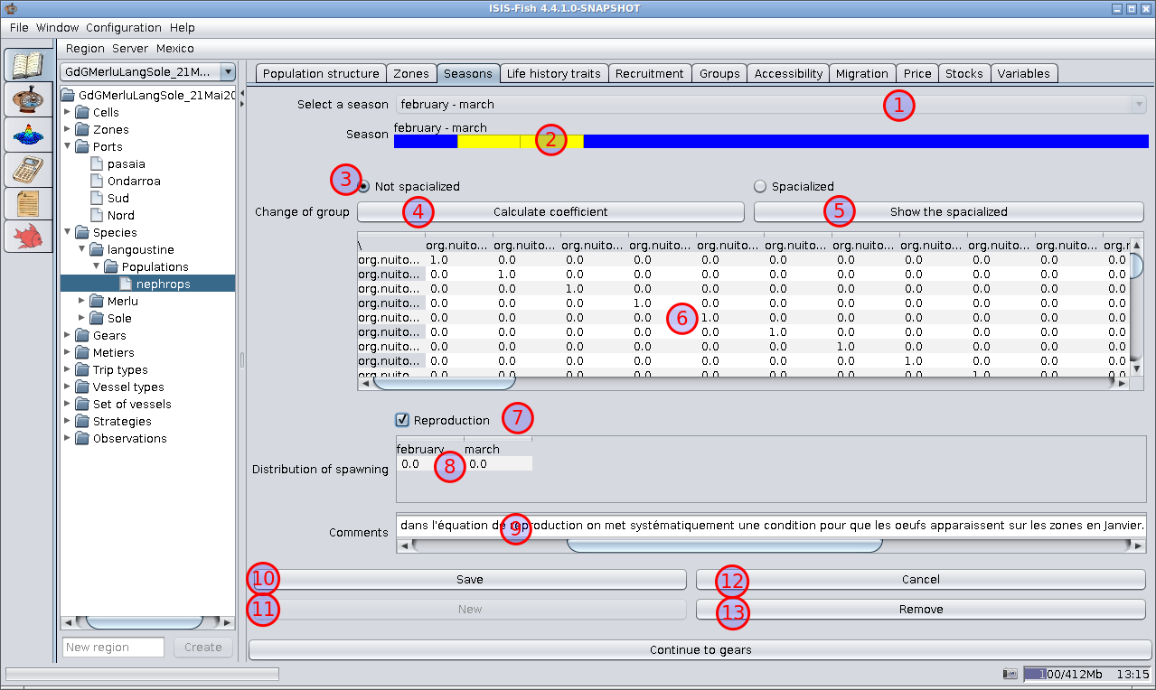
Seasons tab (population structured by length)
The layout of the Seasons tab depends on whether the population is structured by age or length.
-
Select a season – A list of all seasons currently defined for the population
-
Season – The season is shown in yellow. The start and end of the season can be adjusted by dragging the ends of
the bar using the mouse, the whole season can be moved by dragging the middle.
-
Not spacialized / Spatialized – Selects whether the age or length group change coefficients are spatially
independent or spatially dependent.
-
Calculate coefficient – Calculates the coefficient.
-
Show the spatialized (Show spatialized coefficients) – Pops up a window with the spatialized coefficient matrix.
-
Age or length group change coefficient matrix – The coefficients are the fraction of individuals changing from one
age or length group (rows) to another age or length group (columns).
If the matrix is spatially dependent, the number of columns will be equal to the product of the number of age or
length groups and the number of zones in the population area.
Double click on a cell to set the coefficient. Changes to a cell do not take effect until you press Enter or click
another cell in the matrix. Changes to the matrix should be saved using the Save button.
-
Reproduction – Checked if the fish spawn in the season. If it is checked, the “Distribution of spawning” matrix
will be displayed.
-
Distribution of spawning – Shows the fraction of the annual spawning that takes place in each month. Double click
on a cell to set the fraction. Changes to a cell do not take effect until you press Enter or click another cell in
the matrix. Changes to the matrix should be saved using the Save button.
-
Comments – This field is used for adding comments linked to the season selected. Each season may have its own
comments.
-
Save – Saves the changes to the season selected. Do not forget to save your changes.
-
New – Creates an empty season with a default range of months and displays it for editing.
-
Cancel – Throws away the modifications made to the season and reverts to the previous version.
-
Remove – Deletes the season. N.B. The delete operation is irreversible. Once a season has been deleted, it cannot be recovered.
Life history traits tab
The life history traits tab is used to define the equations describing the natural death rate, the mean weight, the
maturity ogive and the reproduction rate for the population.
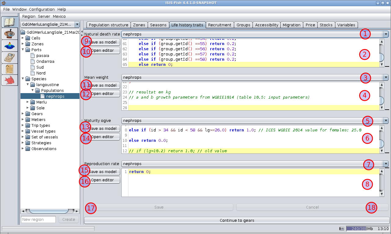
- Drop down list of all previously defined Natural death rate equations for this species.
- Natural death rate equation – The equation can be edited directly in this frame.
- Drop down list of all previously defined Mean weight equations for this species.
- Mean weight equation – The equation can be edited directly in this frame.
- Drop down list of all previously defined Maturity ogive equations for this species.
- Maturity ogive equation – The equation can be edited directly in this frame.
- Drop down list of all previously defined Reproduction rate equations for this species.
- Reproduction rate equation – The equation can be edited directly in this frame. This equation is not always used,
but can be called from scripts and other equations
- Save as model (Natural death rate equation) – Saves the natural death rate equation as a model in the ISIS-Fish
scripts – this can be useful if the equation can be reused for other populations.
- Open editor (Natural death rate equation) – Opens the equation editor for editing the natural death rate equation.
- Save as model (Mean weight equation) – Saves the mean weight equation as a model in the ISIS-Fish scripts – this
can be useful if the equation can be reused for other populations.
- Open editor (Mean weight equation) – Opens the equation editor for editing the mean weight equation.
- Save as model (Maturity ogive equation) : Saves the maturity ogive equation as a model in the ISIS-Fish scripts –
this can be useful if the equation can be reused for other populations.
- Open editor (Maturity ogive equation) – Opens the equation editor for editing the maturity ogive equation.
- Save as model (Reproduction rate equation) – Saves the reproduction rate equation as a model in the ISIS-Fish
scripts – this can be useful if the equation can be reused for other populations.
- Open editor (Reproduction rate equation) – Opens the equation editor for editing the reproduction rate equation.
- Save – Saves the changes to the equations. Do not forget to save your changes.
- Cancel – Throws away the modifications made to the equations and reverts to the previous version.
Recruitment tab
This tab is used to define the reproduction and recruitment for the population.
The reproduction equation is used to calculate the number of eggs released as a equation of the number of reproductive
fish, the fecundity, the age or length group, etc.
The recruitment is defined by a delay to the start of recruitment and the fraction of larvae recruited in each of the
following months. This takes account of the natural variability of the eggs and larvae in a cohort spawned in a given
month. By default, all the individuals in a cohort are recruited in the same month.
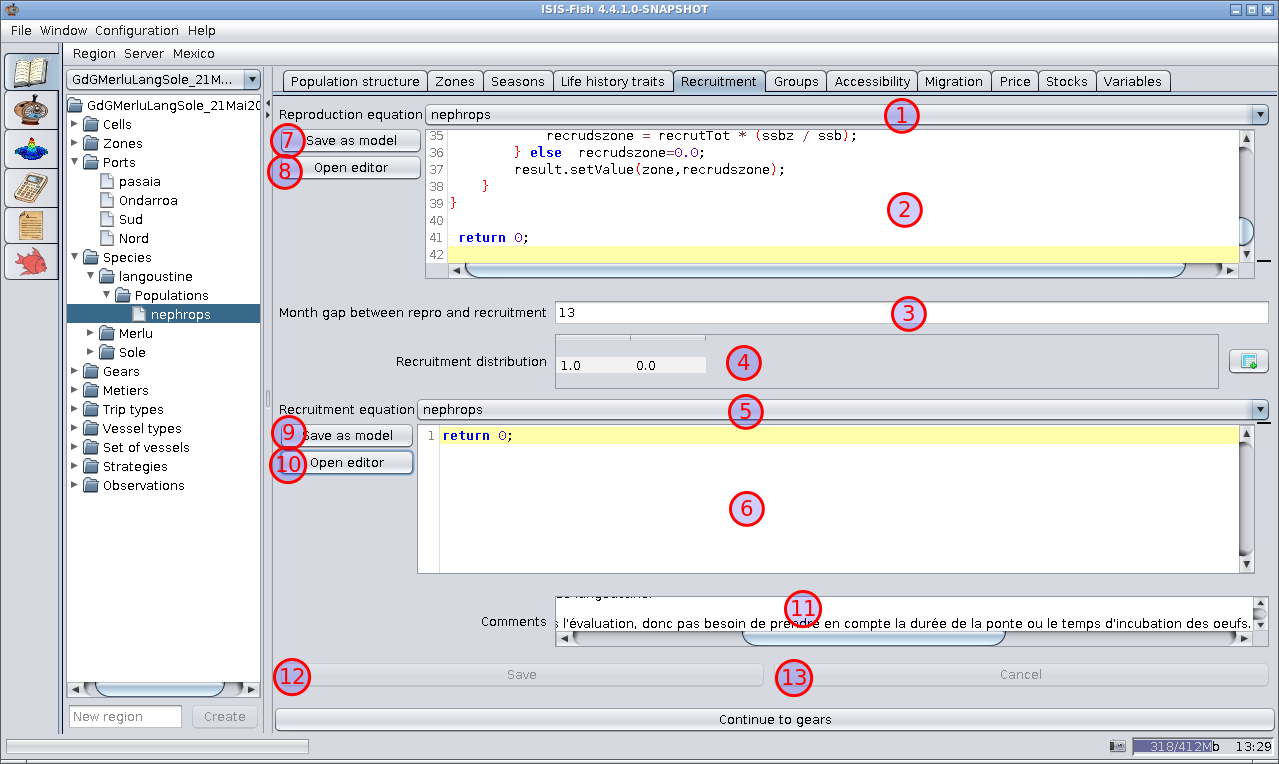
- Drop down list of all previously defined Reproduction equations in the region.
- Reproduction equation – The equation can be edited directly in this frame.
- Month gap between repro and recruitment (Delay from spawning to the start of recruitment) – The number of months
between spawning and the first month in the distribution of recruitment, item 4. This may be zero, in which case the
juveniles are recruited in the same month that the eggs are released (ex for eggs released in June, if the delay is
zero, then the juveniles are recruited in June).
- Recruitment distribution – Matrix with the distribution of the recruitment each month after the start of
recruitment.
- Drop down list of all previously defined Recruitment equations in the region.
- Recruitment equation – The equation can be edited directly in this frame.
- Save as model (Reproduction equation) – Saves the reproduction equation as a model in the ISIS-Fish scripts –
this can be useful if the equation can be reused for other species.
- Open editor (Reproduction equation) – Opens the equation editor for editing the reproduction equation.
- Save as model (Recruitment equation) – Saves the recruitment equation as a model in the ISIS-Fish scripts – this
can be useful if the equation can be reused for other species.
- Open editor (Recruitment equation) – Opens the equation editor for editing the recruitment equation.
- Comments – This field is used for adding comments linked to the equations. Each set of equations may have its own
comments.
- Save – Saves the changes to the reproduction and recruitment. Do not forget to save your changes.
- Cancel – Throws away the modifications made to the reproduction and recruitment and reverts to the previous
version.
Groups tab
This tab is used to visualize the properties of each age or length groups and add comments.
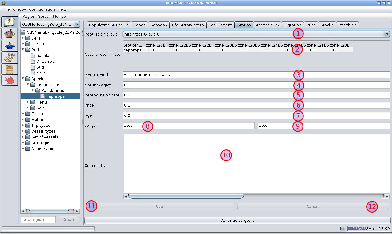
- Drop down list of all age or length groups defined for the population (population structure tab).
- Natural death rate – This table is filled using the natural death rate equation (life history traits tab).
- Mean weight – The mean weight of the group is calculated using the mean weight equation (life history traits tab).
- Maturity ogive – The maturity ogive for the group is calculated using the maturity ogive equation (life history
traits tab).
- Reproduction rate – The reproduction rate for the group is calculated using the reproduction rate equation
(recruitment tab).
- Price – The mean price of the fish in the group value is calculated using the price equation (price tab).
- Age – If the population is structured by age, then the minimum and maximum ages for the group are displayed – if
the population is structured by length, then this is the average age.
- Length – If the population is structured by length, then the minimum and maximum lengths for the group are
displayed – if the population is structured by age, then this is the average length.
- Length – If the population is structured by length, then the minimum and maximum lengths for the group are
displayed – if the population is structured by age, then this is the average length.
- Comments – This field is used for adding comments linked to the age or length group. Each age or length clgroupss
may have its own comments.
- Save – Saves the changes to the comments on the age or length group. Do not forget to save your changes.
- Cancel – Throws away the modifications made to the comments on the age or length group and reverts to the
previous version.
Accessibility tab
The accessibility is defined as probability that an individual will be caught by non-selective fishing gear, for a
standard unit of fishing effort. The accessibility is defined for each combination season and age or length group.
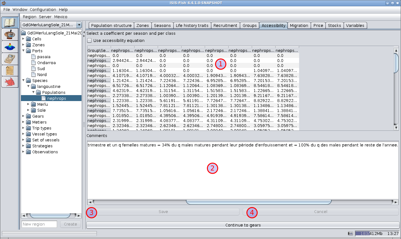
- Matrix of accessibility coefficients – Double click on a cell to set the coefficient. Changes to a cell do not
take effect until you press Enter or click another cell in the matrix. Changes to the matrix should be saved using the
Save button.
- Comments – This field is used for adding comments linked to the accessibility matrix.
- Save – Saves the changes to accessibility matrix. Do not forget to save your changes.
- Cancel – Throws away the modifications made to the accessibility matrix and reverts to the previous version.
Migration tab
This tab is used to define migration within the region and emigration from and immigration into the region, for each
season.
Migration is considered to be instantaneous at the start of the season (see various papers about ISIS-Fish).
Migration can be defined by :
- defining the fraction or size of each age or length group that migrates to and from particular zones;
- defining equations for calculating the migrations.
Population migration sub-tab
This sub tab is used to define the fractions of the population migrating between zones within a region.
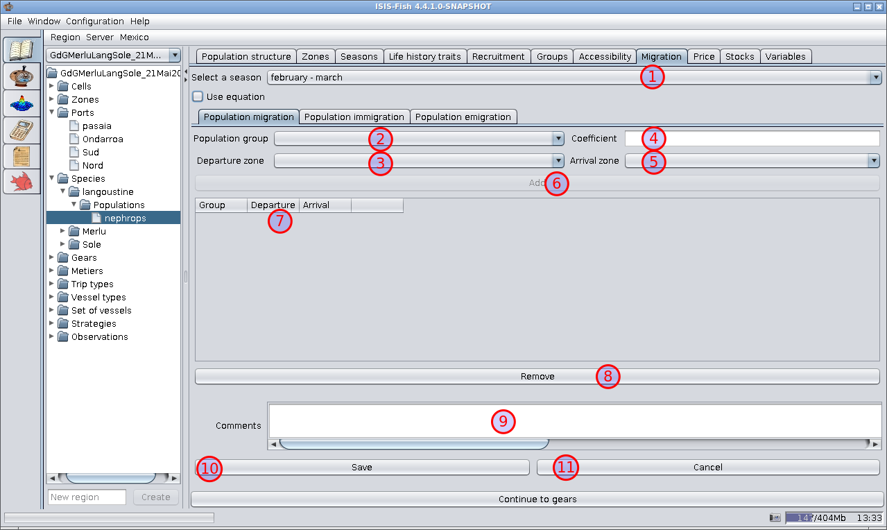
- Select a season – Drop down list of seasons defined for the population: select a season for defining the
migration.
- Population group – The migration is defined separately for each age or length group. The age or length group
should be selected from this list of all groups defined for the population.
- Departure zone – Drop down list for selecting the departure zone from the zones defined for the region.
- Coefficient – The fraction of the age or length group in the departure zone / in the whole population that
migrates.
- Arrival zone – Drop down list for selecting the arrival zone from the zones defined for the region.
- Add – This button adds or overwrites the migration coefficient for the season, the age or length group and
arrival and departure zones. The new coefficient will appear in the matrix below.
- Summary matrix – This matrix summarizes all the migration coefficients currently defined for the season. The
coefficients can be modified directly in this matrix. Double click on a cell to set the coefficient. Changes to a cell
do not take effect until you press Enter or click another cell in the matrix. Changes to the matrix should be saved
using the Save button.
- Remove – Deletes a coefficient from the matrix. First click a row in the matrix to select it and then click
Remove. N.B. The delete operation is irreversible. Once a coefficient has been deleted, it cannot be recovered.
- Comments – This field is used for adding comments linked to the migration, immigration and emigration data for
the population.
- Save – Saves the changes to the migration, immigration and emigration data for all seasons. Do not forget to save
your changes.
- Cancel – Throws away the modifications made to the migration, immigration and emigration data and reverts to the
previous version.
The values of the coefficients should be positive and less than or equal to 1, but there are no validity checks and, for
example, a value of 1000 may be (but should not be) specified without raising an error.
Population immigration sub-tab
This sub tab is used to define the numbers immigrating into each zone from outside the region.
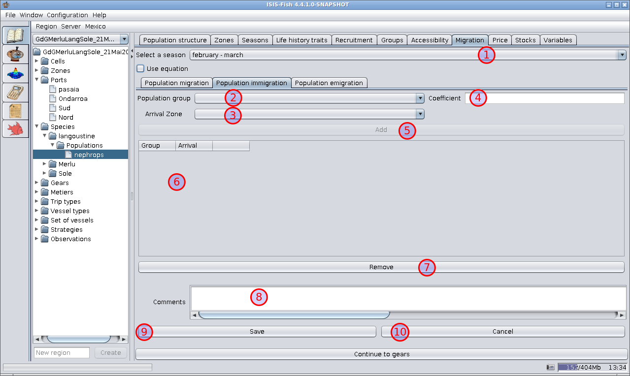
- Select a season – Drop down list of seasons defined for the population: select a season for defining the
immigration.
- Population group – The immigration is defined separately for each age or length group. The age or length group
should be selected from this list of all groups defined for the population.
- Arrival zone – Drop down list for selecting the arrival zone from the zones defined for the region.
- Number – The count of immigrant individuals in the age or length group.
- Add – This button adds or overwrites the immigration count for the season, the age or length group and arrival
zone. The new count will appear in the matrix below.
- Summary matrix – This matrix summarizes all the immigration counts currently defined for the season. The counts can
be modified directly in this matrix. Double click on a cell to set the count. Changes to a cell do not take effect
until you press Enter or click another cell in the matrix. Changes to the matrix should be saved using the Save button.
- Remove – Deletes an immigration count from the matrix. First click a row in the matrix to select it and then click
Remove. N.B. The delete operation is irreversible. Once a count has been deleted, it cannot be recovered.
- Comments – This field is used for adding comments linked to the migration, immigration and emigration data for
the population.
- Save – Saves the changes to the migration, immigration and emigration data for all seasons. Do not forget to
save your changes.
- Cancel – Throws away the modifications made to the migration, immigration and emigration data and reverts to the
previous version.
There are no validity checks on the counts.
Population emigration sub-tab
This sub tab is used to define the fractions of the population emigrating from each zone within a region.
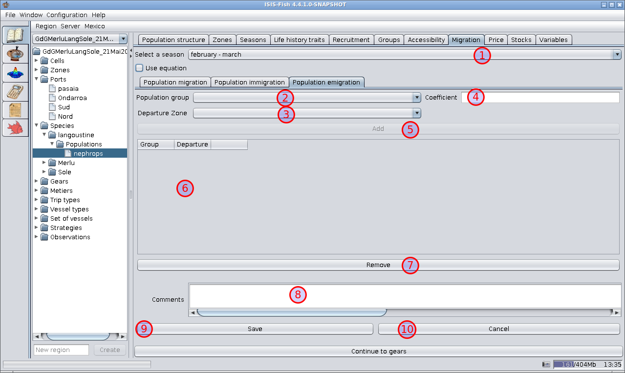
- Select a season – Drop down list of seasons defined for the population: select a season for defining the
emigration.
- Population group – The emigration is defined separately for each age or length group. The age or length group
should be selected from this list of all groups defined for the population.
- Departure zone – Drop down list for selecting the departure zone from the zones defined for the region.
- Coefficient – The fraction of the age or length group in the departure zone / in the whole population that
emigrates.
- Add – This button adds or overwrites the emigration coefficient for the season, the age or length group and
arrival zone. The new coefficient will appear in the matrix below.
- Summary matrix – This matrix summarizes all the emigration coefficients currently defined for the season. The
coefficients can be modified directly in this matrix. Double click on a cell to set the coefficient. Changes to a cell
do not take effect until you press Enter or click another cell in the matrix. Changes to the matrix should be saved
using the Save button.
- Remove – Deletes a coefficient from the matrix. First click a row in the matrix to select it and then click
Remove. N.B. The delete operation is irreversible. Once a coefficient has been deleted, it cannot be recovered.
- Comments – This field is used for adding comments linked to the migration, immigration and emigration data for
the population.
- Save – Saves the changes to the migration, immigration and emigration data for all seasons. Do not forget to
save your changes.
- Cancel – Throws away the modifications made to the migration, immigration and emigration data and reverts to the
previous version.
The values of the coefficients should be positive and less than or equal to 1, but there are no validity checks and, for
example, a value of 1000 may be (but should not be) specified without raising an error.
Population migration defined using equations
This menu appears if the Use equation checkbox is checked.
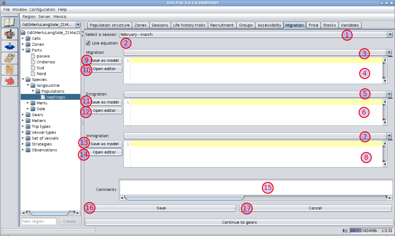
- Select a season – Drop down list of seasons defined for the population: select a season for defining the
migration, immigration or emigration.
- Use equation – This box should be checked if the migration, immigration and emigration are to be defined using
equations.
- Migration equation selector – Selects a equation for defining migration from those already defined for the
region.
- Migration equation – Displays the migration equation. The equation may be edited in this frame.
- Immigration equation selector – Selects a equation for defining immigration from those already defined for the
region.
- Immigration equation – Displays the immigration equation. The equation may be edited in this frame.
- Emigration equation selector – Selects a equation for defining emigration from those already defined for the
region.
- Emigration equation – Displays the emigration equation. The equation may be edited in this frame.
- Save as model (Migration equation) – Saves the migration equation as a model in the ISIS-Fish scripts – this can
be useful if the equation can be reused for other species.
- Open editor (Migration equation) – Opens the equation editor for editing the migration equation.
- Save as model (Immigration equation) – Saves the immigration equation as a model in the ISIS-Fish scripts – this
can be useful if the equation can be reused for other species.
- Open editor (Immigration equation) – Opens the equation editor for editing the immigration equation.
- Save as model (Emigration equation) – Saves the emigration equation as a model in the ISIS-Fish scripts – this
can be useful if the equation can be reused for other species.
- Open editor (Emigration equation) – Opens the equation editor for editing the emigration equation.
- Comments – This field is used for adding comments linked to the migration, immigration and emigration data for
the population.
- Save – Saves the changes to the migration, immigration and emigration data for all seasons. Do not forget to save
your changes.
- Cancel – Throws away the modifications made to the migration, immigration and emigration equations and reverts to
the previous version.
7. Define the fishing gear
There are two tabs for defining fishing gear
- Gear :Defines the general characteristics of the fishing gear.
- Selectivity : Defines an equation representing the selectivity of the fishing gear.
Gear tab
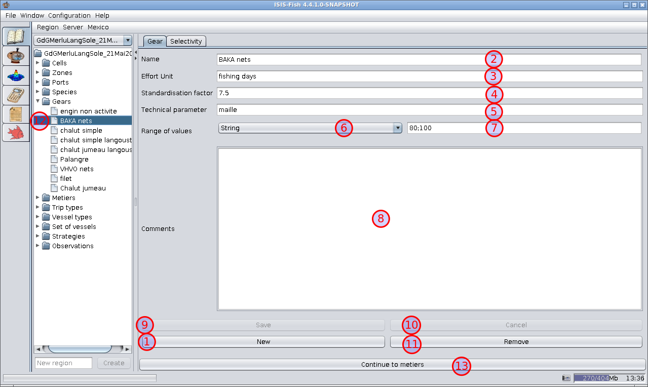
- New – Creates an empty fishing gear definition with the name “Gear_new”, adds it to the object tree and displays it for editing.
- Name – The name of the fishing gear (as it is the name of the fishery object, it is a good idea to standardize the name, e.g. using alphanumeric characters and avoiding punctuation).
- Effort units – The units used to define the fishing effort.
- Standardisation factor – A positive floating point number used to normalize the fishing effort for different fishing gears.
- Technical parameter – A parameter used to characterize the fishing gear (mesh, number of hooks, etc.). This may be used to calculate the selectivity or it may be used in a rule. It must, therefore, conform to Java naming conventions.
- Type (Range of values) – Sets the type of the values in the range of values.
- Range (Range of values) – Defines the range of possible values. The values may be specified conventionally as a semicolon separated list (e.g. “10;30;50” or “small;medium;large”) or as a continuous range with the lower and upper limits separated by a hyphen (e.g. “10-50”).
- Comments – This field is used for adding comments linked to the fishing gear selected. Each type of fishing gear may have its own comments.
- Save – Saves the changes to the fishing gear selected. Do not forget to save your changes.
- Cancel – Throws away the modifications made to the fishing gear and reverts to the previous version.
- Remove – Deletes the fishing gear. N.B. The delete operation is irreversible. Once a fishing gear definition has been deleted, it cannot be recovered.
- Fishing gear in the object tree – the type of fishing gear to be modified must be selected in the object tree.
- Continue to metiers – To move on to the next step either click Continue to metiers or select Metiers in the object tree.
Selectivity tab
A selectivity equation must be defined for each population that might be caught by the fishing gear.
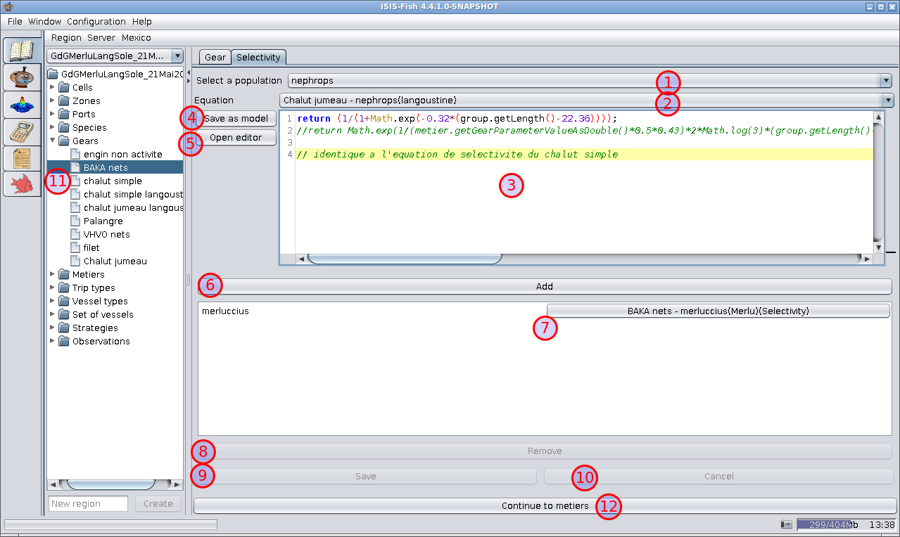
-
Select a population – A list of all populations currently defined for the region.
-
Drop down list of all previously defined Selectivity equations for the region. When the type of fishing gear is
saved, the equations defined for the gear (if they are new equations) are added to this list. If the selectivity
equation required is similar, or identical, to a selectivity equation that has already been used for another
population or fishing gear, select it from this list.
-
Selectivity equation – The equation can be edited directly in this frame.
-
Save as model – Selectivity equation) – Saves the selectivity equation as a model in the ISIS-Fish scripts – this
can be useful if the equation can be reused elsewhere.
-
Open editor – Selectivity equation) – Opens the equation editor for editing the fishing gear selectivity
equation.
-
Add – This button adds the selectivity equation for the population to the type of fishing gear.
-
Table of Selectivity equations. This table lists all the populations for which selectivity equations have been
defined for the fishing gear.
You can open the equation editor for a selectivity equation by clicking the right hand button.
-
Remove – Deletes a selectivity equation from the fishing gear. First click a row in the table to select it and
then click Remove.
-
Save – Saves the changes to the selectivity equations. Do not forget to save your changes.
-
Cancel – Throws away the modifications made to the selectivity equations and reverts to the previous version.
-
Fishing gear in the object tree – the type of fishing gear to be modified must be selected in the object tree.
-
Continue to metiers – To move on to the next step either click Continue to metiers or select Metiers in
the object tree.
8. Define the “metiers”
The “métier”, the use of a particular configuration of fishing gear, in particular seasons, in a particular area is
defined using three tabs.
- Metier : Defines the name and fishing gear used.
- Season / zones : Defines the fishing zones for each season for the metier.
- Catchable species : Defines the species that may be caught.
Metier tab
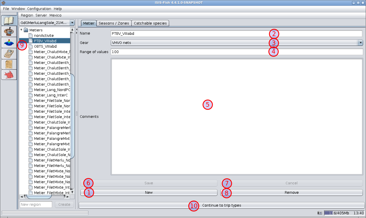
- New – Creates an empty metier definition with the name “Metier_new”, adds it to the object tree and displays it
for editing.
- Name – The name of the metier (as it is the name of the fishery object, it is a good idea to standardize the
name, e.g. using alphanumeric characters and avoiding punctuation).
- Gear – A list of all the types of fishing gear defined for the region. Select the fishing gear to be used for
the metier.
- Gear parameter – The value of the parameter used to characterize the fishing gear (mesh, number of hooks, etc.).
This should be with the range of values specified for the fishing gear.
- Comments – This field is used for adding comments linked to the metier selected. Each metier may have its own comments.
- Save – Saves the changes to the metier selected. Do not forget to save your changes.
- Cancel – Throws away the modifications made to the metier and reverts to the previous version.
- Remove – Deletes the metier. N.B. The delete operation is irreversible. Once a metier definition has been
deleted, it cannot be recovered.
- Metier in the object tree – the type of metier to be modified must be selected in the object tree.
- Continue to trip types – To move on to the next step either click Continue to trip types or select
Trip types in the object tree.
Seasons / zones tab
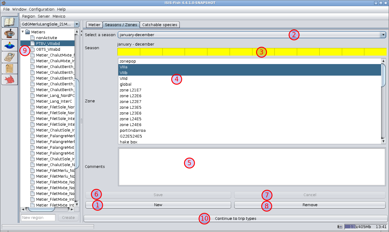
- New – Creates a new season, and its associated fishing zones, for the metier.
- Select a season – A list of all seasons currently defined for the metier.
- Season – The season is shown in yellow. The start and end of the season can be adjusted by dragging the ends of
the bar using the mouse, the whole season can be moved by dragging the middle.
- Zone – Select a single fishing zone by clicking the name. Select a group of zones by clicking the first zone,
pressing Shift and clicking the last zone, select or unselect individual zones by pressing Ctrl and clicking the
zone.
- Comments – This field is used for adding comments linked to the season selected. Each season may have its own
comments.
- Save – Saves the changes to the season definition selected. Do not forget to save your changes.
- Cancel – Throws away the modifications made to the season definition and reverts to the previous version.
- Remove – Deletes the season definition. N.B. The delete operation is irreversible. Once a season definition has
been deleted, it cannot be recovered.
- Metier in the object tree – the type of metier for which the seasons are to be defined must be selected in the object
tree.
- Continue to trip types – To move on to the next step either click Continue to trip types or select
Trip types in the object tree.
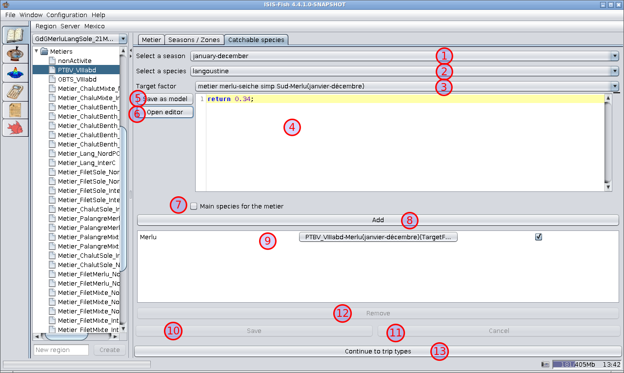
Catchable species tab
-
Select a season – A list of all seasons defined in the Seasons / zones tab.
-
Select a species – A list of all species currently defined for the region.
-
Drop down list of all previously defined target factors for the region.
-
Target factor – The equation can be edited directly in this frame.
-
Save as model (Target factor) – Saves the target factor equation as a model in the ISIS-Fish scripts – this can
be useful if the equation can be reused elsewhere.
-
Open editor (Target factor) – Opens the equation editor for editing the target factor equation.
-
Main species for the metier – Checkbox to mark this species as the main target for the metier.
-
Add – This button adds the species ad its target factor equation to the season.
-
Matrix of target factor equations. This matrix lists all the species and their target factor equations that have been
defined for the season and metier.
You can open the equation editor for a target factor equation by clicking the central button.
-
Save – Saves the changes to the catchable species. Do not forget to save your changes.
-
Cancel – Throws away the modifications made to the catchable species and reverts to the previous version.
-
Remove – Deletes a target factor equation from the fishing gear. First click a row in the matrix to select it and
then click Remove.
-
Continue to trip types – To move on to the next step either click Continue to trip types or select
Trip types in the object tree.
There are no coherence checks for the target equation and multiple target equations may be (but should not be) defined
for a given season and species without raising an error.
9. Define the types of trip
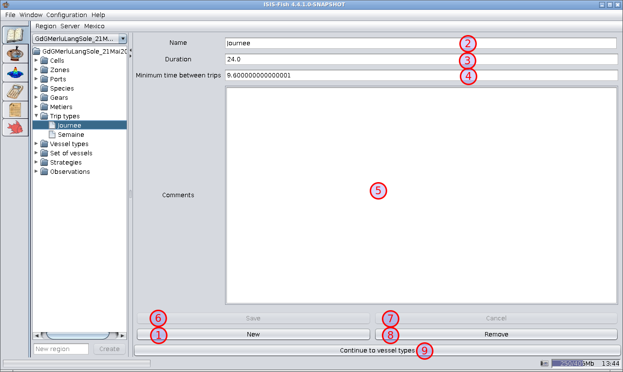
- New – Creates an empty type of trip with the name “TripType_new”, adds it to the object tree and displays it for
editing.
- Name – The name of the type of trip (as it is the name of the fishery object, it is a good idea to standardize
the name, e.g. using alphanumeric characters and avoiding punctuation).
- Duration – The duration of the trip in hours.
- Minimum time between trips – The minimum time between two trips in days.
- Comments – This field is used for adding comments linked to the type of trip selected. Each type of trip may have
its own comments.
- Save – Saves the changes to the type of trip selected. Do not forget to save your changes.
- Cancel – Throws away the modifications made to the type of trip and reverts to the previous version.
- Remove – Deletes the type of trip. N.B. The delete operation is irreversible. Once a type of trip has been
deleted, it cannot be recovered.
- Continue to vessel types – To move on to the next step either click Continue to vessel types or select
Vessel types in the object tree.
10. Define the types of vessel
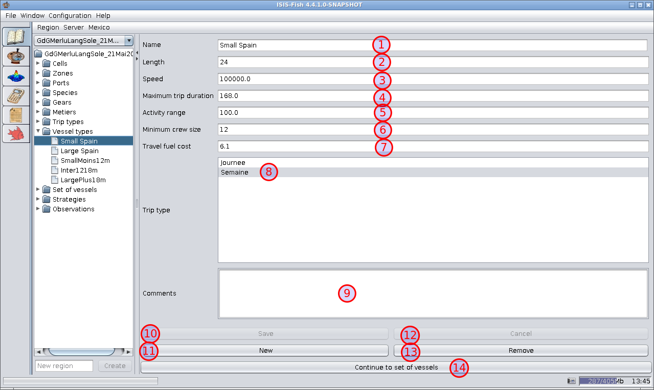
- Name – The name of the type of vessel (as it is the name of the fishery object, it is a good idea to standardize
the name, e.g. using alphanumeric characters and avoiding punctuation).
- Length – Typical length of this type of boat (meters).
- Speed – Average speed of this type of boat (Km/hours).
- Maximum trip duration – The maximum length of a fishing trip (hours).
- Activity range – ????
- Minimum crew size – The smallest possible crew (persons).
- Travel fuel cost – The fuel cost used for calculation the cost of a trip (per hour AND NOT PER KM).
- Trip type – This matrix lists all the types of trip defined for the region. At least one type of trip must be
selected. Select a group of types of trip by clicking the first type of trip, pressing Shift and clicking the last
type of trip, select or unselect individual types of trip by pressing Ctrl and clicking the type of trip.
- Comments – This field is used for adding comments linked to the type of vessel selected. Each type of vessel may
have its own comments.
- Save – Saves the changes to the type of vessel selected. Do not forget to save your changes.
- New – Creates an empty type of vessel with the name “VesselType_new”, adds it to the object tree and displays it
for editing.
- Cancel – Throws away the modifications made to the type of vessel and reverts to the previous version.
- Remove – Deletes the type of vessel. N.B. The delete operation is irreversible. Once a type of vessel has been
deleted, it cannot be recovered.
- Continue to set of vessels – To move on to the next step either click Continue to set of vessels or select
Set of vessels in the object tree.
11. Define the sets of vessels
A set of vessels of a similar type and pursuing a similar strategy is defined using three tabs.
- Characteristics – Defines general characteristics of the set of vessels.
- Metiers – Defines the metiers used by the vessels.
- Metier parameters – Defines the parameters for each metier.
Characteristics tab
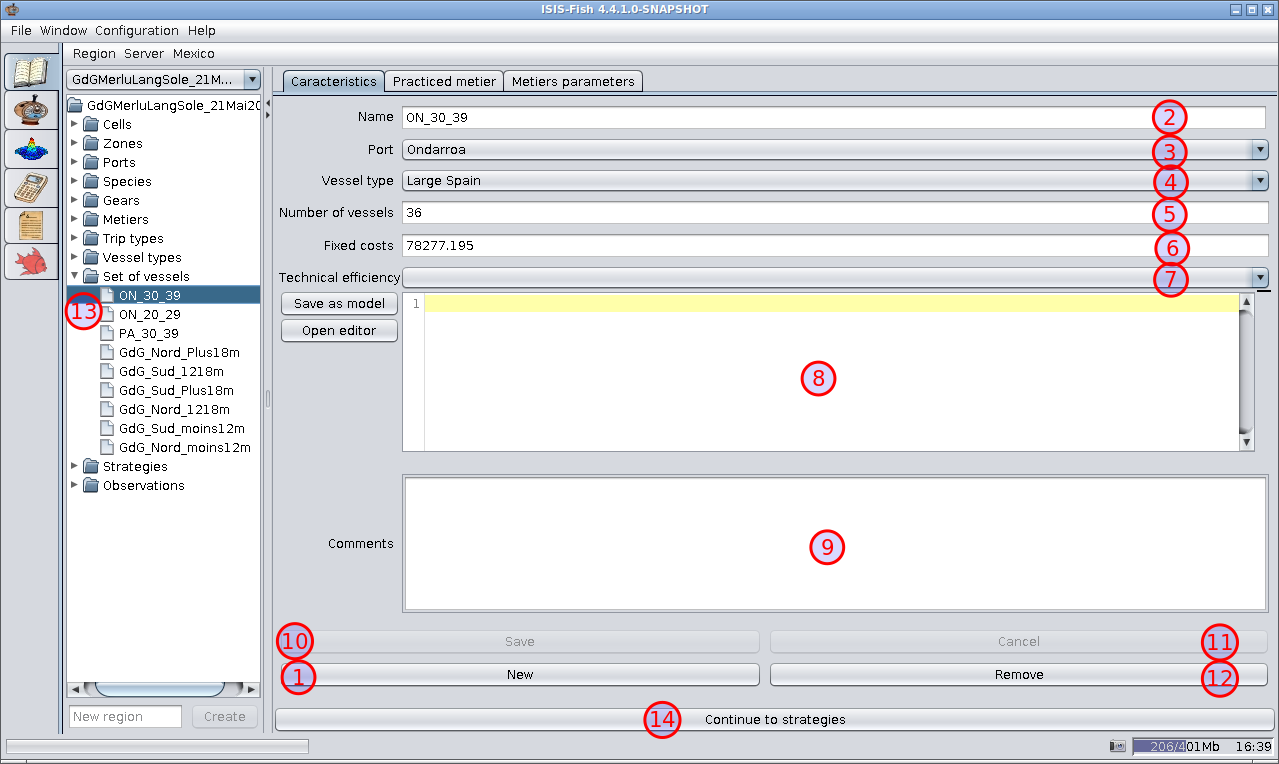
- New – Creates an empty set of vessels definition with the name “SetOfVessels_new”, adds it to the object tree and
displays it for editing.
- Name – The name of the set of vessels (as it is the name of the fishery object, it is a good idea to standardize
the name, e.g. using alphanumeric characters and avoiding punctuation).
- Port – Defines the home port for the set of vessels.
- Vessel type – Drop down list of all the types of vessel defined for the region. One vessel must be selected.
- Number of vessels – Defines the number of vessels in the set.
- Fixed costs – The fixed costs of operating the vessel (€ / year).
- Drop down list of all Efficiency equations previously defined for ???
- Efficiency equation – The equation can be edited directly in this frame.
- Comments – This field is used for adding comments linked to the set of vessels selected. Each set of vessels may
have its own comments.
- Save – Saves the changes to the set of vessels selected. Do not forget to save your changes.
- Cancel – Throws away the modifications made to the set of vessels and reverts to the previous version.
- Remove – Deletes the set of vessels. N.B. The delete operation is irreversible. Once a set of vessels has been
deleted, it cannot be recovered.
- Set of vessels in the object tree – the type of set of vessels to be modified must be selected in the object tree.
- Continue to strategies – To move on to the next step either click Continue to strategies or select
Strategies in the object tree.
Practiced metier tab
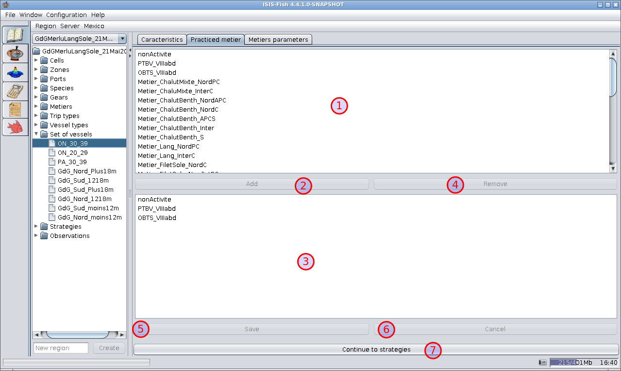
- List of all metiers defined for the region.
- Add – Adds the metiers selected in the list, item 1, to the list of metiers for the set of vessels, item 3. N.B.
Avoid adding the same metier more than once.
- List of all the metiers associated with the set of vessels.
- Remove – Removes the selected metiers from the list of metiers item 3.
- Save – Saves the changes to the set of vessels. Do not forget to save your changes.
- Cancel – Throws away the modifications made to the set of vessels and reverts to the previous version.
- Continue to strategies – To move on to the next step either click Continue to strategies or select
Strategies in the object tree.
Metier parameters tab
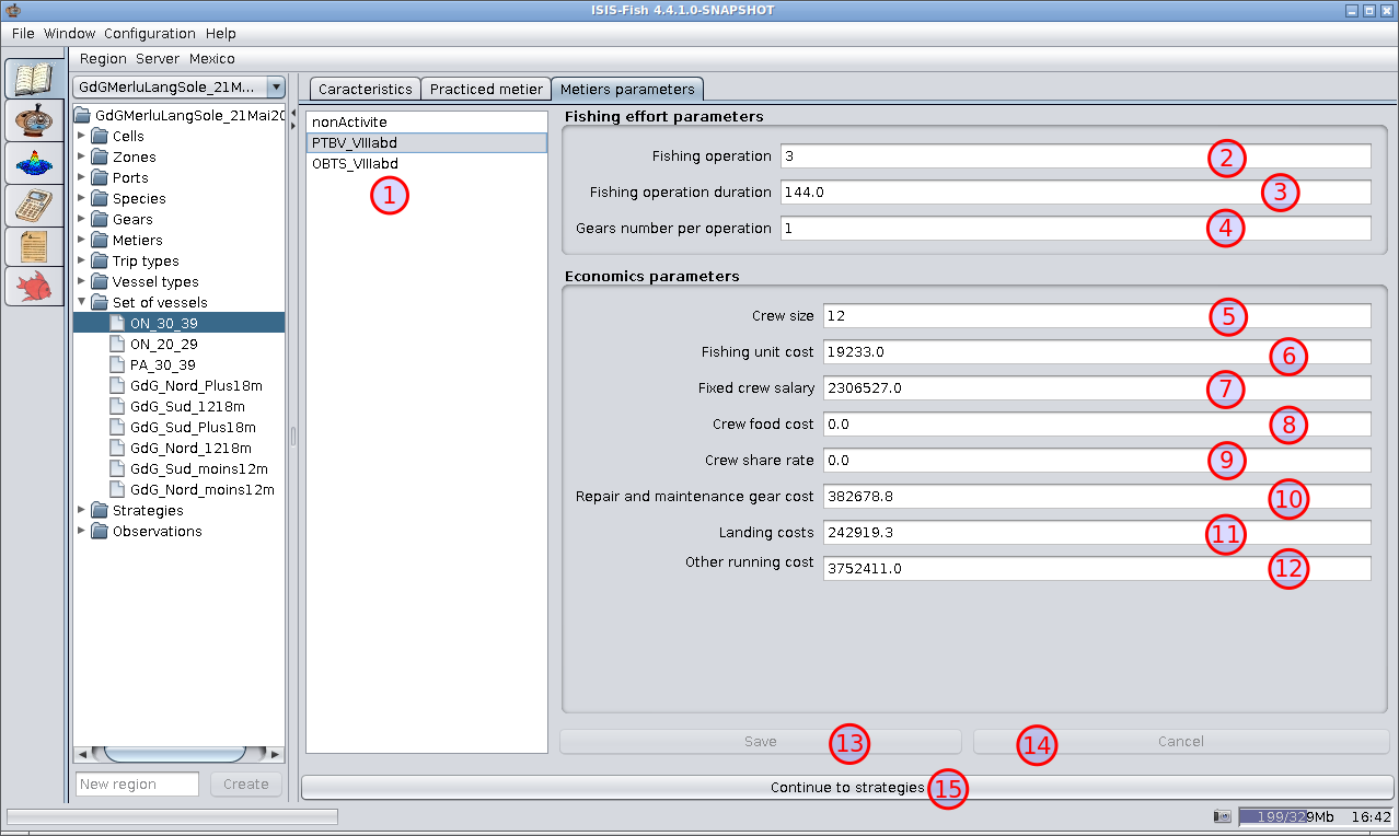
- List of all metiers defined for the set of vessels. Select the metier to be parameterized.
- Fishing operations – Defines the number of fishing operations per day for this metier and set of vessels.
- Fishing operation duration – Defines the length of each fishing operation for this metier and set of vessels
(hours).
- Gears per operation – Defines the number of fishing gears deployed for this metier and set of vessels.
- Crew size – The number of crew members for this metier and set of vessels.
- Fishing unit cost – The cost of each fishing operation in terms of fuel, oil and ice for this metier and set of
vessels (€).
- Fixed crew salary – The basic wage cost for the crew for this metier and set of vessels (€ / month).
- Crew food cost – The basic food cost for the crew for this metier and set of vessels (???).
- Crew share rate – The crew share in addition to the fixed crew costs, item 7.
- Repair and maintenance gear cost (Gear maintenance cost) – The fishing gear repair and maintenance costs
(€ / day).
- Landing costs – The landing fees payable to the home port for this metier and set of vessels.
- Other running costs – Any other operating costs for this metier and set of vessels (€ / hour).
- Save – Saves the changes to the metier parameters. Do not forget to save your changes.
- Cancel – Throws away the modifications made to the metier parameters and reverts to the previous version.
- Continue to strategies – To move on to the next step either click Continue to strategies or select
Strategies in the object tree.
The cost parameters do not need to be specified for carrying out a simulation. A simulation using only the biological
model can be run with all cost parameters set to zero (the default).
12. Define the strategies
The fishing strategies are defined using two tabs.
- Characteristics – Defines general characteristics of the strategy.
- StrategyMonthInfo – Defines the monthly breakdown of the strategy.
Characteristics tab
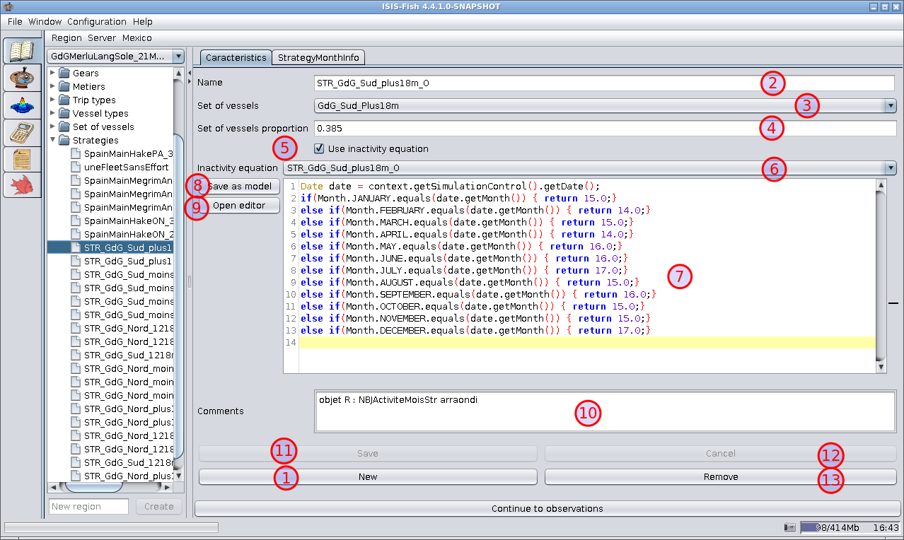
- New – Creates an empty fishing gear definition with the name “Strategy_new”, adds it to the object tree and
displays it for editing.
- Name – The name of the strategy (as it is the name of the fishery object, it is a good idea to standardize the
name, e.g. using alphanumeric characters and avoiding punctuation).
- Sets of vessels – A dropdown list of all sets of vessels defined for the region. Select one.
- Sets of vessels proportion – Defines the fraction of the set of vessels that follows this strategy.
- Use inactivity equation – This box should be checked to specify inactivity periods using an equation.
- Inactivity equation selector – A list of inactivity equations defined for the region.
- Inactivity equation – Displays the inactivity equation. The equation may be edited in this frame.
- Save as model (inactivity equation) – Saves the inactivity equation as a model in the ISIS-Fish scripts – this can
be useful if the equation can be reused for other species.
- Open editor (Inactivity equation) – Opens the equation editor for editing the inactivity equation.
- Comments – This field is used for adding comments linked to the strategy selected. Each type of strategy may have
its own comments.
- Save – Saves the changes to the strategy selected. Do not forget to save your changes.
- Cancel – Throws away the modifications made to the strategy and reverts to the previous version.
- Remove – Deletes the strategy. N.B. The delete operation is irreversible. Once a strategy has been deleted, it
cannot be recovered.
StrategyMonthInfo tab
This tab is used to define the strategy for each month. There are twelve groups of fields to define the type of trip and
number of days of inactivity each month and a matrix to specify the proportion of the each month devoted to each metier.
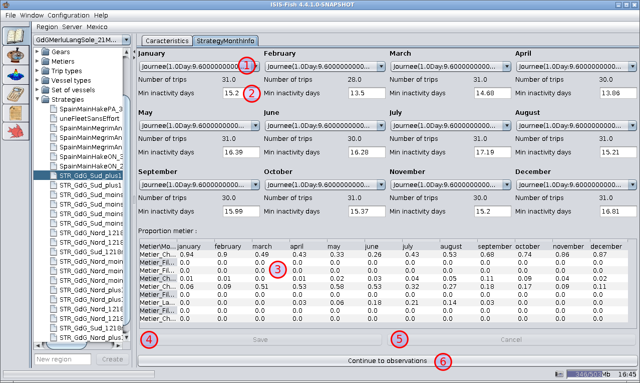
- Type of trip – A dropdown list of all the types of trip defined for the region. A single type of trip must be
selected.
- Min inactivity days – Defines the minimum number of days of inactivity.
- Proportion metier – Specifies the fraction of the time spent each month on each metier associated with the set
of vessels.
- Save – Saves the changes to the strategy selected. Do not forget to save your changes.
- Cancel – Throws away the modifications made to the strategy and reverts to the previous version.
- Continue to observations – To move on to the next step either click Continue to observations or select
Observations in the object tree.
13. Add observations
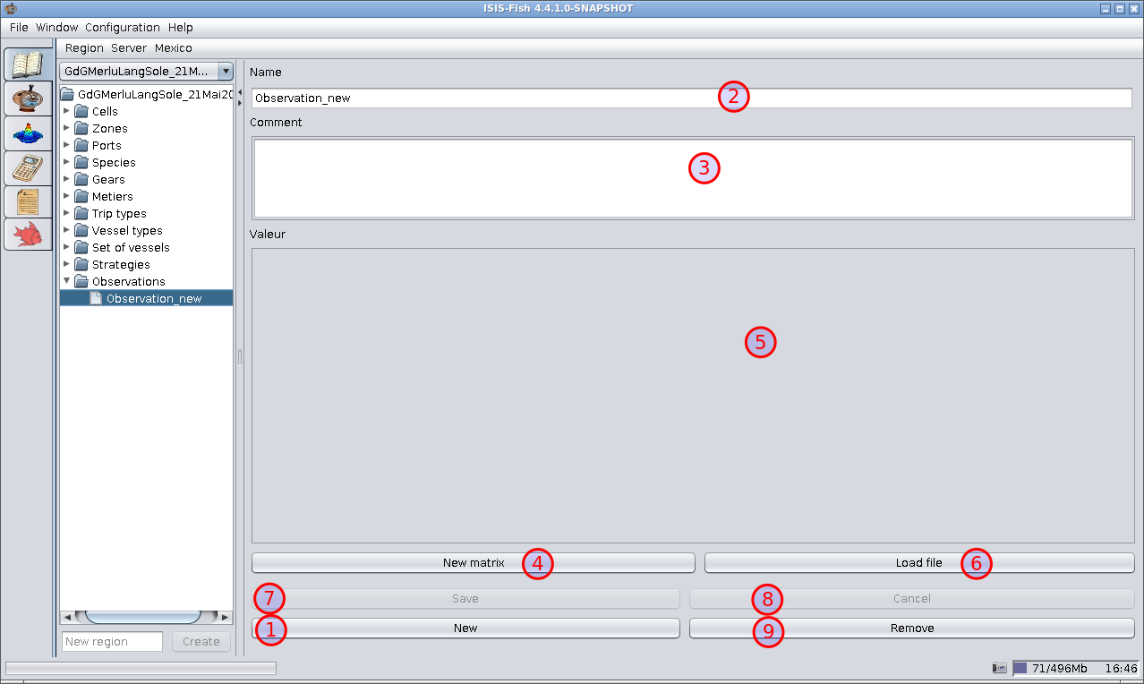
- New – Creates an empty observation with the name “Observation_new”, adds it to the object tree and displays it
for editing.
- Name – The name of the observation (as it is the name of the fishery object, it is a good idea to standardize the
name, e.g. using alphanumeric characters and avoiding punctuation).
- Description – Description of the observation.
- New matrix – Opens a dialogue box for creating an empty matrix. The dimensions should be specified as rowscolumns
(e.g. 49).
- Observed values – The observed values. Double click on a cell to set a value. Changes to a cell do not take
effect until you press Enter or click another cell in the matrix. Changes to the matrix should be saved using the
Save button.
- Load file – Loads a file with the observations.
- Save – Saves the changes to the observation selected. Do not forget to save your changes.
- Cancel – Throws away the modifications made to the observation and reverts to the previous version.
- Remove – Deletes the observation. N.B. The delete operation is irreversible. Once an observation has been
deleted, it cannot be recovered.