


 This module is used to create, launch and use the results of a sensitivity analysis.
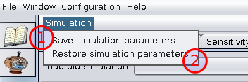
The menus carry out global actions for the sensitivity analysis.
A sensitivity analysis involves a number of stages.
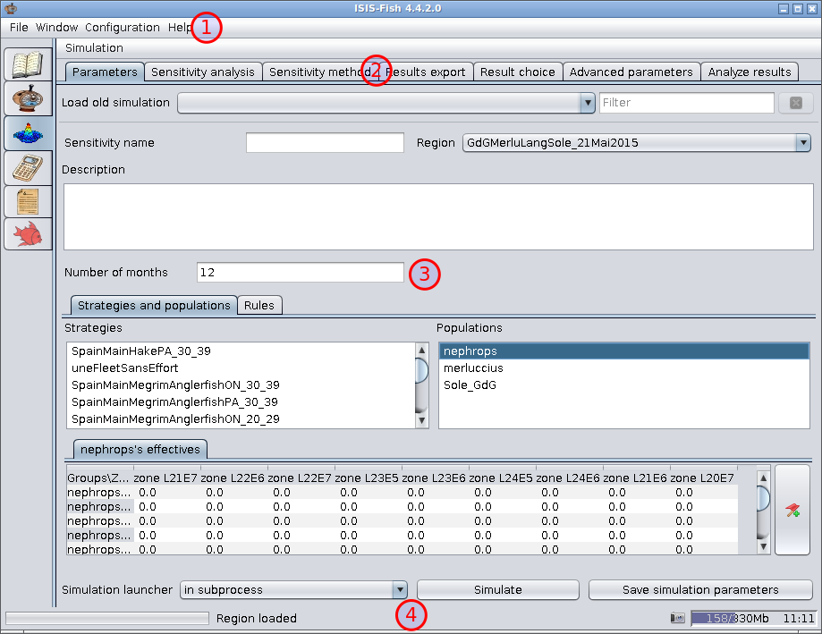
The Parameters tab is used for setting the basic simulation parameters.
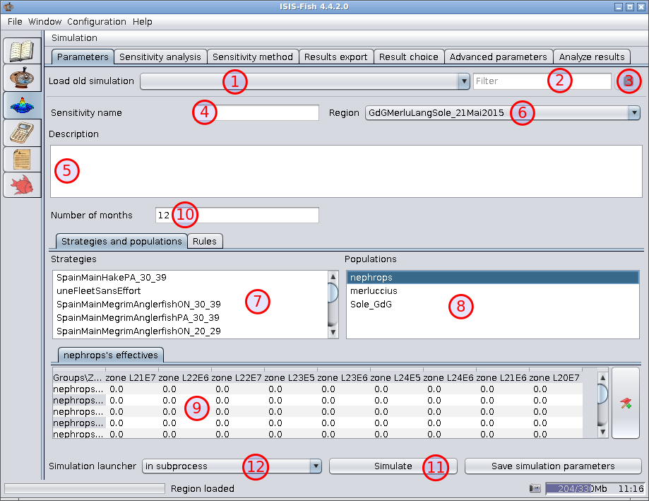
Load old simulation – This lists all the simulations executed locally. The list is empty when ISIS-Fish is executed for the first time. When a simulation is run successfully, it will be added to this list the next time ISIS-Fish is run.
Filter – Filter for the list of simulations.
Refresh list (to the right of the filter) – Cancels the current simulation filter and refreshes the list of simulations.
Sensitivity name – The name of the sensitivity analysis.
If you load a previous simulation, the name will appear here.
A new simulation can be created easily from a previous simulation by changing the name.
Description – The description of the sensitivity analysis.
If you load a previous simulation, the description will appear here.
Region – Select the region for the sensitivity analysis.
Loading the region will fill in the list of strategies and the list of populations.
Always select the region before defining the rules as these are linked to the objects in the region.
Strategies – When the region has been loaded, all the strategies defined for the region will be listed here. The strategies selected in this list will be used by the simulator.
Populations – When the region has been loaded, all the populations defined for the region will be listed here.
When a population is selected, the initial counts for age or length groups in each population zone are displayed in the table, Item 9.
These are used to initialize the simulator.
Initial population – This table holds the initial counts for each age or length group in each zone for the population selected.
Number of months – This specifies the period over which the simulation is carried out.
Simulate – Runs the simulation as specified by Simulation launcher.
Simulation launcher – Specifies where the simulations will be run:
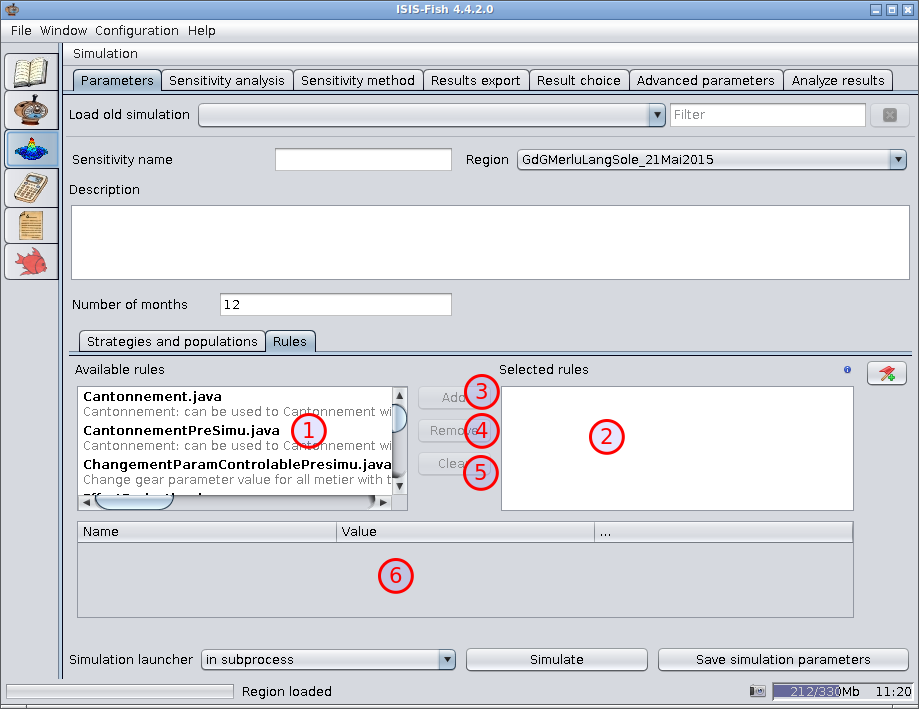
Available rules – This is a list of rules that have been defined in ISIS-Fish. Each rule is followed by its description.
Selected rules – This is the list of rules that have been selected for the simulation. Each rule is followed by its description.
When a rule is selected in this list, the parameters are displayed in the table below.
Add – Adds the rules selected in the Available rules, Item 10, to the Selected rules, Item 11. As each rule is added, a dialog box is displayed for setting the parameters.
Remove – Removes the rules selected from the Selected rules, Item 11.
Clear – Removes all the rules from the Selected rules, Item 11.
Rule parameters – When a rule in the Selected rules list is selected, the parameters are displayed in this table and may be modified.
When you move the pointer over a parameter name, a tooltip will appear with the description of the parameter.
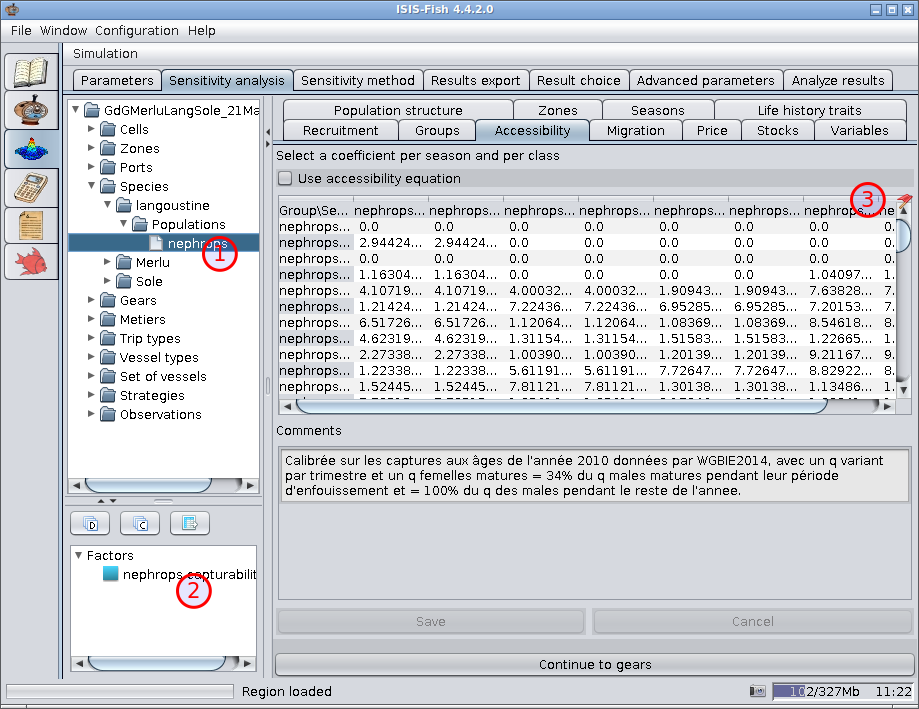
The sensitivity analysis tab has the object tree for the region for select objects and their parameters that will be used as factors in the sensitivity analysis.
Object tree for the region – For selecting an object with one or more parameters to be used as factors.
Factors that have been selected – As each factor is selected it is added to this list.
Double clicking a factor opens the dialog box for setting the parameters for the factor. A right click opens a context menu for deleting the factor
Parameter that can be used as a factor – This icon indicates the parameter can be used as a factor. It is animated to indicate that the pointer is hovering over the field for potential factor. Clicking the field opens a dialog box for setting the parameters for the factor.
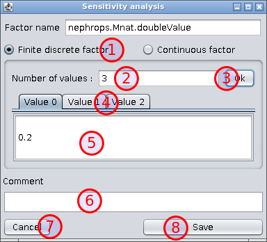
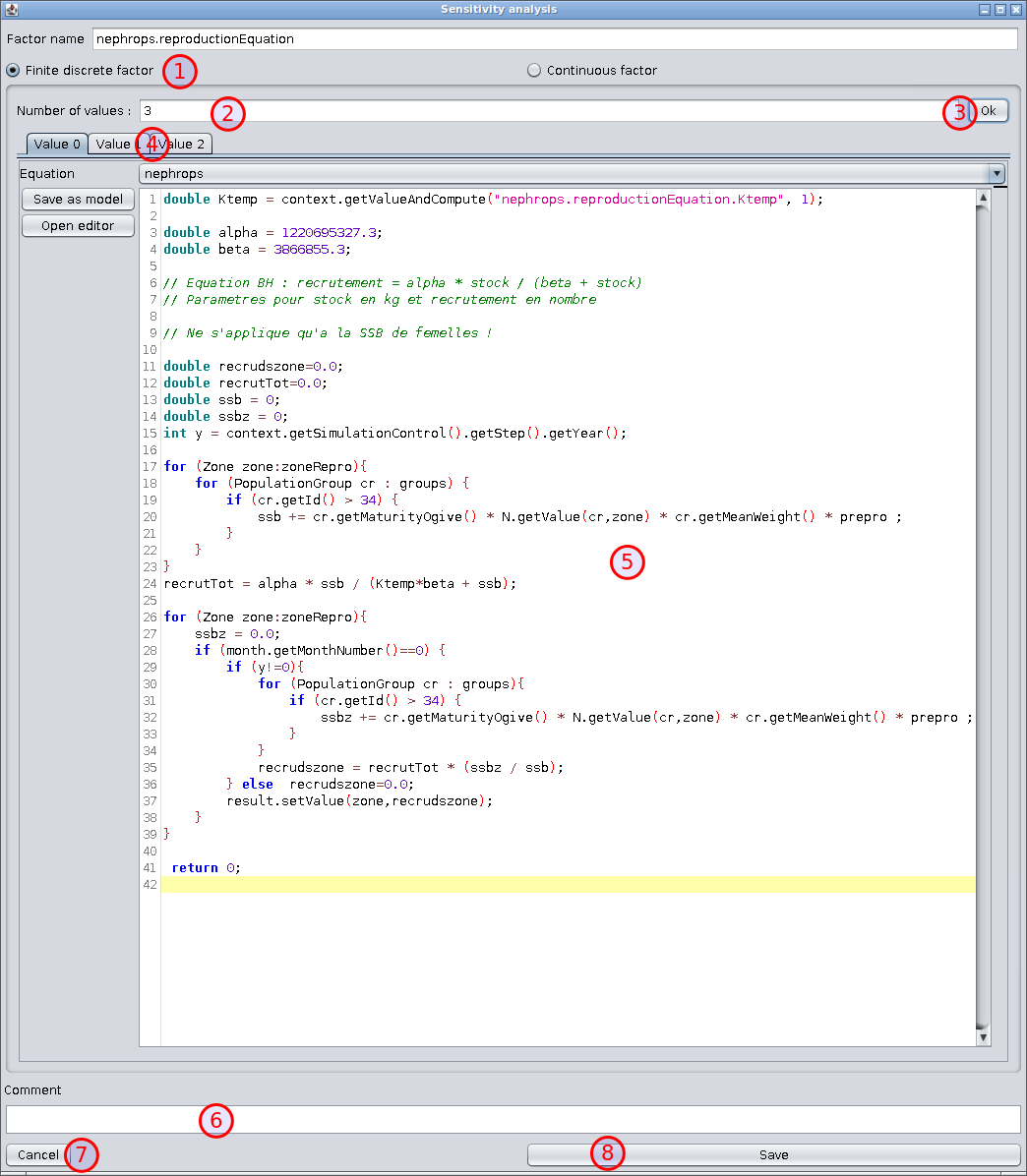
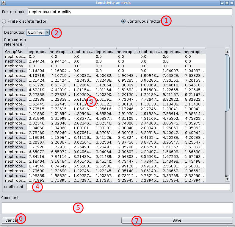
When a parameter defined as a value is used as a factor, the value may either be continuously variable or be one of a set of discrete values. For a continuously variable factor, the distribution must be specified.
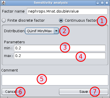
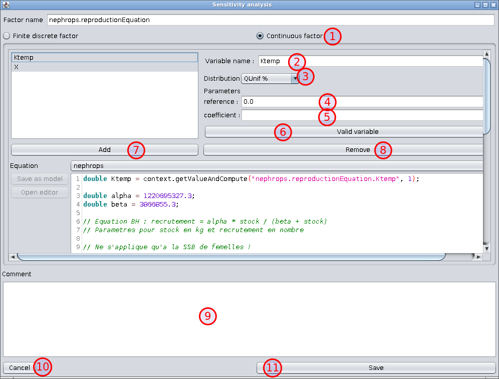
Continuous factor – Selected if the factor is continuously variable.
Variable name – The variable should be a constant in the equation. When the factor is defined the line in the equation defining the constant is modified so that the value can be changed during the analysis. Note. If the factor is a variable that exists only for sensitivity analysis, then this variable should be added to the equation with a default value (e.g. double Ktemp = 1) and the equation changed to use this value.
Distribution – Dropdown list of probability distributions.
First parameter – The first parameter for the distribution selected – Reference for QUnif%, usually the default in the equation.
Last parameter – The last parameter for the distribution selected – Coefficient for QUnif%.
Valid variable – Checks that the constant is defined in the equation, modifies the equation to vary this constant and saves the parameters. The modification to the equation does not affect its use in other simulations that may be carried out.
A single equation may have a factor for any or all of the constants in the equation. ISIS-Fish will create a
factor for each constant added in this dialogue box.
Add – Adds a new factor.
Remove – Removes the factor selected.
Comment – Any useful information about the factor or factors.
Cancel – Throw away the modifications made. If the dialogue box was opened to create a new factor, then no new factors will be created.
Save – Saves the parameters for the factor or factors. If the dialogue box was opened to create a new factor, the new factor or factors will be added to the list of factors selected.
Remove (not visible when adding a new factor) – Removes the factor from the analysis.

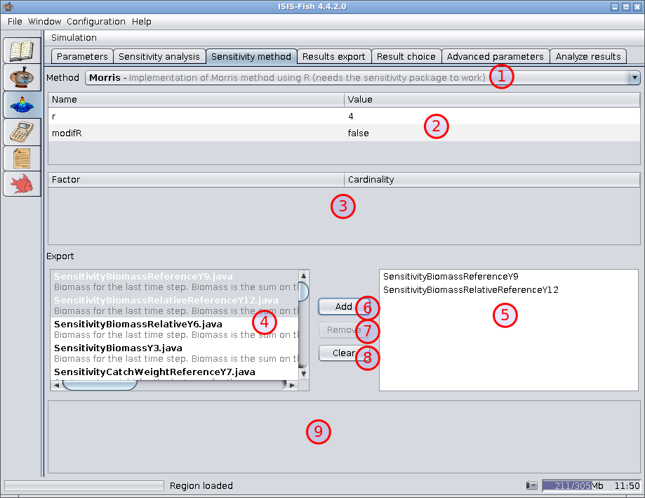
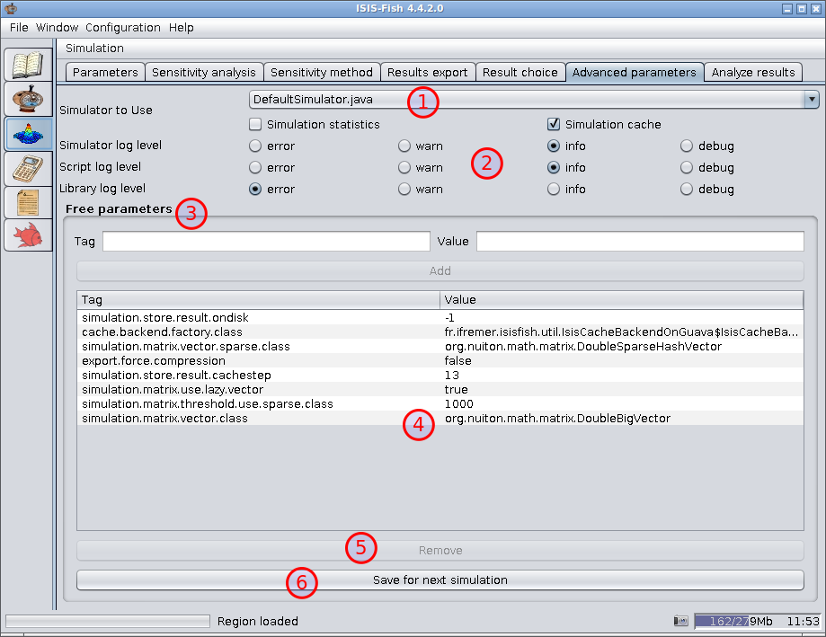
Simulator to use – This sets the basic simulator configuration.
Log filter settings – Sets the log levels for deferent parts of ISIS-Fish.
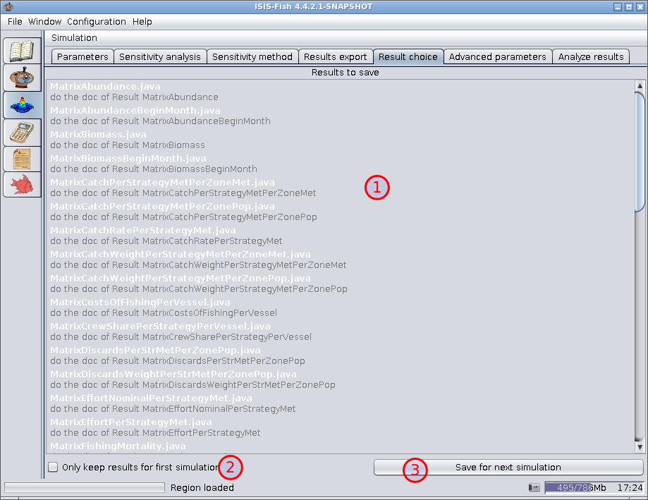
Free parameters – The top part of the Free parameters frame is used to define new free parameters. After setting the Tag and the Value, click Add to add the parameter to the list, Item 4.
Free parameter list – This lists all the free parameters that have been defined
Remove – Removes the free parameter selected (if one is selected) from the list.
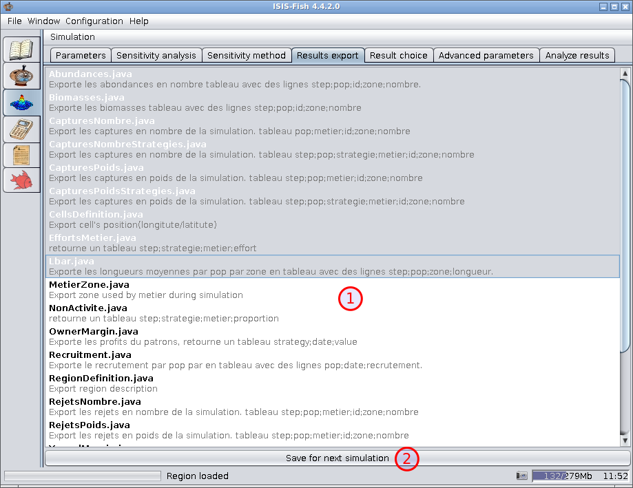
Save for next simulation – saves the settings so that the next time the simulation launcher is run, the settings will be reloaded.
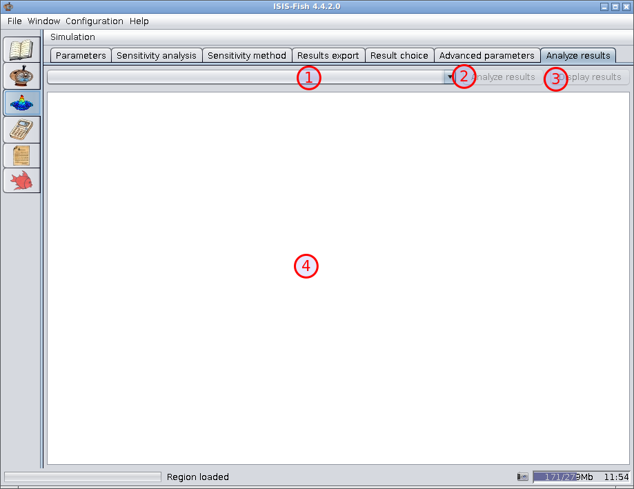
List of sensitivity analysis – A list of all the sensitivity analyses known. N.B. This may include analyses that have not yet been carried out.
Analyze results – Run the analysis scripts on the results of the simulations and display the analysis in the analysis frame.
|tip| The results are always analyzed after the last simulation has terminated. This button reruns the analyses on the results of the simulations without having to rerun the simulations themselves. The means that the sensitivity analysis scripts can be modified after the simulations have been run.
Display results – Display the results of the sensitivity analysis.
Analysis frame – Displays the results of the sensitivity analysis. Only those results that are exported by the sensitivity analysis scripts are shown.
The sensitivity analysis scripts use R for the calculations. The objects used are standard and the R session is saved. The results can, therefore, be used in R for further processing.
The results are in the SensitivityAnalysisName.RData file in the isis-export directory defined in the
configuration file.
The .RData file holds a session with numerous R objects from the various sensitivity analysis stages.
isis.factorisis.factor is a 5 column, single row data frame.
nomFacteurNominal (value in the database)Continu (TRUE/FALSE)Binf (minimum value)Bsup (maximum value if continuous, otherwise the number of values)Attributes
nomFacteur: list(values)nomModel: “isis-fish-externeR”isis.factor is registered in R as SensitivityAnalysisName_0.isis.factor (all spaces are stripped by R).
isis.factor.distributionisis.factor.distribution is a 3 column data frame with one row per factor
NomFacteurNomDistributionParametreDistributionisis.factor.distribution is registered in R as SensitivityAnalysisName_0.isis.factor.distribution (all spaces
are stripped by R).
isis.methodExpisis.methodExp is a list with three objects
isis.factorisis.factor.distributioncallAttributes
nomModel: “isis-fish-externeR”isis.methodExp is registered in R as SensitivityAnalysisName_0.isis.methodExp (all spaces are stripped by R).
isis.simuleisis.simule is a data frame with one row per simulation and one column for each factor and each simulation result
Attributes
nomModel: “isis-fish-externeR”call: the method that generating the simulations.isis.simule is registered in R as SensitivityAnalysisName_0.isis.simule (all spaces are stripped by R).
isis.methodAnalyseisis.methodAnalyse is a list with 5 objects:
isis.factorisis.factor.distributionisis.simulecall_methodanalysis_result (R object with the analysis results. If the results were calculated by aov, the object
is a list with the aov and the sensitivity indices.)isis.methodAnalyse is registered in R as SensitivityAnalysisName_0.ResultName.isis.methodAnalyse (all spaces are stripped by R).
You can always use the R function ls() to list all the objects in the R session.